The first week tackled the implementation of different kind of linear regression for the creation of the last layer in the Echo State Network. More specifically were added the possibility to add a \( l_1 \) regularization to the loss function (Lasso regression), both \( l_1 \) and \( l_2 \) regularizations (Elastic Net regression) and also added the possibility to choose the Huber loss function. As in the last post we will start from a brief theoretical background to explain the code and then we will showcase some examples taken from the literature.

Theoretical Background

In the Brief Introduction to Reservoir Computing we showed how it was possible to get the output layer from a linear regression over the states and the desired output using Ridge regression:

$$\textbf{W}_{\text{out}} = \textbf{Y}^{\text{target}} \textbf{X}^{\text{T}}(\textbf{X} \textbf{X}^{\text{T}} + \beta \textbf{I})^{-1}$$ but by doing so we actually jumped a few steps, and in the example it wasn’t even used actually, it was just an Ordinary Least Squares(OLS). To know the difference we have to take a little step back. Inherently generalised linear regression models are an optimisation problem of the form

$$L(\textbf{y}, \textbf{X} \theta)+P(\theta)$$

where

• \( \textbf{y} \) is the target
• \( \textbf{X} \) is the design matrix
• \( \theta \) is a vector of coefficient to determine
• \( L \) is a loss function
• \( P \) is a penalty function

OLS and penalization

In the case of Ridge regression the loss function is the OLS, to wich is added a \( l_2 \) regularization. The function to minimize is of the form

$$||\textbf{y} - \textbf{X} \theta ||_2^2 + \lambda || \theta ||_2^2$$

where \( ||.||_2 \) is the \( l_2 \) norm and \( \lambda \) is a penalization coefficient. In the Lorenz system example the lambda parameter was set to zero so in fact we were actually fitting using only the first part of the above expression, that corresponds to OLS, as said before. The formula we showed in the opening is actually quite different from this second definition, but this is because even though this is an optimisation problem the Ridge regression has a closed form solution. So if we imagine to have a matrix of targets \(\textbf{Y}\) and \(\theta = \textbf{W}_{\text{out}} \) then the first definition can be derived from the second.

Another form of regression based on the OLS loss function is Lasso (least absolute shrinkage and selection operator) which uses the \( l_1 \) norm as regularization. The function to minimize will hence have the form

$$||\textbf{y} - \textbf{X} \theta ||_2^2 + \lambda || \theta ||_1$$

This two methods can be linearly combined in order to obtain the Elastic Net regression method, of the form

$$||\textbf{y} - \textbf{X} \theta ||_2^2 + \lambda || \theta ||_2^2 + \gamma || \theta ||_1$$

This last two methods, contrarily to Ridge regression, do not present a closed form and so one has to use other solutions to the optimization problem, such as gradient descent or proximal gradient method.

Huber loss function

Of course one can choose other alternatives to the OLS loss function, and one of the most common is the Huber loss function. Used in robust regression is known to respond well in the presence of outliers. The function is defined as follows

$$L_{\sigma}(a) = \frac{1}{2}a^2 \text{ for } |a| \le \sigma$$ $$L_{\sigma}(a) = \sigma (|a| - \frac{1}{2} \sigma ) \text{ otherwise}$$

To this function we can apply the same regularization function priorly defined, the \( l_2 \) and \( l_1 \) norm if one so choses.

Implementation in ReservoirComputing.jl

The implementation in the library has been done leveraging the incredible job done by the MLJLinearModels.jl team. The ESNtrain() function can now take as argument the following structs:

• Ridge(lambda, solver)
• Ridge(lambda, solver)
• ElastNet(lambda, gamma, solver)
• RobustHuber(delta, lambda, gamma, solver)

where lambda gamma and delta are defined in the theoretical sections above and solver is a solver of the MLJLinearModels library. One must be careful to use the suitable solver for every loss and regularization combination. Further information can be found in the MLJLinearModels documentation.

Examples

The Lasso regression was first proposed in [1] and in [2] a variation is proposed on it and there are also comparison with Elastic Net regression. Other comparison are carried out in [3], which is the paper we will follow as methodology. The Huber loss function is used for comparison in [4], but to my knowledge has not been adopted in other papers.

Trying to follow the data preparation used in [3] we use the Rossler system this time to carry out our tests. The system is defined by the equations $$\frac{dx}{dt} = -y -z$$ $$\frac{dy}{dt} = x + ay$$ $$\frac{dz}{dt} = b + z(x - c)$$ andit exhibits chaotic behavior for \( a = 0.2 \), \( b = 0.2 \) and \( c = 5.7 \). Using Range Kutta of order 4 from the initial positions \( (-1, 0, 3) \) the time series is generated with step size set to 0.005. In the paper the attractor is reconstructed in the phase space using embedding dimensions \( (3, 3, 3) \) and time delays \( (13, 13, 13) \) for the \(x, y, z\) series respectively. After, all the 9 resulting timeseries are rescaled in the range \( [-1, 1] \) and will all be used in the training of the ESN. Since the data preparation was unusual for me I spent a couple of hours wrapping my head around it. If one wants to know more about time delays and embeddings a good brief introduction is given in [5]. Thankfully DynamicalSystems.jl makes lifes easier when dealing with this type of problems and using embed() I was quickly able to create the data as expressed in the paper. StatsBase.jl dealt with the rescaling part.

The parameter for the ESN are then set as follows

using ReservoirComputing
shift = 100

sparsity = 0.05
approx_res_size = 500
radius = 0.9
activation = tanh
sigma = 0.01
train_len = 3900
predict_len = 1000
lambda = 5*10^(-5)
gamma = 5*10^(-5)
alpha = 1.0
nla_type = NLADefault()
extended_states = true

h = 1

The test was based on a h steps ahead prediction, which differs from the normal prediction because after every h steps of the ESN running autonomosly after training, the actual data is fed into the model, “correcting” the results. This way one has also to feed test data into to model, and the error is consequently quite low. As we can see the h parameter is set on 1, since that is the step used in the paper. The model only predicts one step in the future this way, for every step of the prediction.

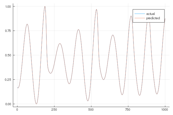
To test the difference between values we used a user-defined Root Mean Square Deviation (RMSE) for the x coordinate, following paper guidelines. The results are as follows, given as a mean of 20 different initiations of random reservoirs:

$$ \text{rmse}_{\text{RESN}} = 9.033 \cdot 10^{-5} $$ $$ \text{rmse}_{\text{LESN}} = 0.006 $$ $$ \text{rmse}_{\text{EESN}} = 0.006 $$ $$ \text{rmse}_{\text{HESN}} = 9.040 \cdot 10^{-5} $$

where RESN is the Ridge regression trained ESN, LESN is the Lasso trained ESN, EESN is the Elastic Net trained ESN and HESN is the ESN trained with Huber function with \( \delta = 0.8\) and \( l_2 \) norm.

We can also take a look at a plot of the x coordinate bot actual and predicted, but as one can expect from a rmse so small there is almost no difference.

The results obtained, while not in line with what is showed in the literature, are actually far better, by several orders of magnitude in some instances. While not obtaining the comparison with the papers is somewhat not optimal, there are some problems with the paper examined: the presence of several blunders in the final published draft, sometimes really evident, do not give ground to the dismissal of results but can raise eyebrows to the transparency of the methods or data utilized. In conclusion, the implementations to the ESN show promising results, but a more thorough exploration and examination needs to be done in order to really showcase their true utility. There will be time for that after GSoC ends, hopefully.

As always, if you have any questions regarding the model, the package or you have found errors in my post, please don’t hesitate to contact me!

Citing

Part of the work done for this project has been published. If this post or the ReservoirComputing.jl software has been helpful, please consider citing the accompanying paper:

@article{JMLR:v23:22-0611,
  author  = {Francesco Martinuzzi and Chris Rackauckas and Anas Abdelrehim and Miguel D. Mahecha and Karin Mora},
  title   = {ReservoirComputing.jl: An Efficient and Modular Library for Reservoir Computing Models},
  journal = {Journal of Machine Learning Research},
  year    = {2022},
  volume  = {23},
  number  = {288},
  pages   = {1--8},
  url     = {http://jmlr.org/papers/v23/22-0611.html}
}

References

[1] Han, Min, Wei-Jie Ren, and Mei-Ling Xu. “An improved echo state network via L1-norm regularization.” Acta Automatica Sinica 40.11 (2014): 2428-2435.

[2] Xu, Meiling, Min Han, and Shunshoku Kanae. “L 1/2 Norm Regularized Echo State Network for Chaotic Time Series Prediction.” International Conference on Neural Information Processing. Springer, Cham, 2016.

[3] Xu, Meiling, and Min Han. “Adaptive elastic echo state network for multivariate time series prediction.” IEEE transactions on cybernetics 46.10 (2016): 2173-2183.

[4] Guo, Yu, et al. “Robust echo state networks based on correntropy induced loss function.” Neurocomputing 267 (2017): 295-303.

[5] http://www.scholarpedia.org/article/Attractor_reconstruction