The second week of the Google Summer of Code project with ReservoirComputing.jl dealt with the implementation of a Support Vector based regression for the Echo State Network model, resulting in the Support Vector Echo-State Machine (SVESM). In this post we will quickly touch on the theory behind Support Vector Regression (SVR), and then we will see the results of the implementation into the library. At the end a couple of examples are given, togheter with a comparison between SVR and SVESMs.
Theoretical Background
Support Vector Regression
What follows is just an overview of the theory behind SVR, which takes for granted a priori knowledge of the reader of the more general concepts of Support Vector Machines. A more knowledgable and in depth exposition can be found in [1] and [2]. Most of the information presented in this section is taken from these papers unless stated otherwise.
In a general setting, a regression task can be expressed as the minimization of the following primal objective function: $$C \sum_{j=1}^{N}L[\textbf{x}_j, y_{dj}, f ] + ||\textbf{w}||^2$$ where
- \(L\) is a general loss function
- \(f\) is the prediction function defined by \(\textbf{W}\) and \(b\)
- \(C\) is a regularization constant
If the loss function is quadratic the objective function can be minimized by means of linear algebra, and the methodology is called Ridge Regression.
The most used function in SVR is called \(\epsilon\)-insensitive loss function [3]:
$$L = 0 \ \text{ if } |f(x)-y| < \epsilon$$ $$L = |f(x)-y| - \epsilon \text{ otherwise }$$
More specifically we can consider the equation
$$\text{min}||\textbf{w}||^2+C\sum_{j=1^{N_t}}(\xi _j+\hat{\xi}_j)$$
with constraints (for \(j=1,…,N_t\)): $$(\textbf{w}^T \textbf{x}_j+b)-y_j \le \epsilon - \xi_j$$ $$y_j-(\textbf{w}^T \textbf{x}_j+b) \le \epsilon - \xi_j$$ $$\xi _j,\hat{\xi}_j \ge 0$$
the solution of which can be found using the following dual problem
$$\text{min}_{\alpha , \alpha^*} \frac{1}{2} \sum_{i, j = 1}^{N_t}(\alpha_i-\alpha_i^*)(\alpha_j-\alpha_j^*)\textbf{x}^T\textbf{x}-\sum_{i=1}^{N_t}(\alpha_i-\alpha_i^*) y_i + \sum_{i=1}^{N_t}(\alpha_i-\alpha_i^*) \epsilon$$
with constraints:
$$0 \le \alpha _i, \alpha _i^* \le C, \sum_{i=1}^{N_t}(\alpha_i-\alpha_i^*)=0$$
We can clearly see that to solve this task one has to resort to quadratic programming. The solution will have the form
$$f(\textbf{x}) = \sum_{i=1}^{N_p}(\alpha_i-\alpha_i^*) k(\textbf{x}_i, \textbf{x})$$
where \(k\) is a so-called kernel function, an implicit mapping of the data into an higher dimension, used to turn a non linear problem into a linear one. This is the “kernel trick”, where the mapping is not explicitly done, but is obtained using function that only require the computation of the inner products. Common kernels includes:
- Linear \( k(\textbf{x}_i, \textbf{x}_j) = \textbf{x}_i \cdot \textbf{x}_j\)
- Polynomial \(k(\textbf{x}_i, \textbf{x}_j) = (\textbf{x}_i \cdot \textbf{x}_j)^d \)
- Gaussian Radial Basis Function \( k(\textbf{x}_i, \textbf{x}_j) = e^{ \lambda ||\textbf{x}_i - \textbf{x}_j||^2} \)
Support Vector Echo State Machines
We can see that the intuition behind the Reservoir Computing approach is similar to the kernel methods: using a fixed Recurrent Neural Network (for the case of the ESN) we are also mapping the input into a higher dimension. Therefore the connection between the two models was almost immediate and the idea developed in [4] was to perform a linear SVR in the higer dimensional reservoir state space.
In the paper different loss function are analized: quadratic loss function, \( \epsilon \)-insensitive loss function and the Huber loss function. A new method of prediction is also proposed, called the direct method. This method is a variation of the one step ahead prediction, in which the desired output is not the next step, but a \( h \) steps ahead one. The input-output training sequences can be described as \( \textbf{d}(k), \textbf{x}(k+h), k=1, 2, 3,…, N_t \) where \( \textbf{d}(k) \) is the embedding of the target time series and \( \textbf{x}(k+h) \) is the \( h \) steps ahead target output for training/testing.
Implementation in ReservoirComputing.jl
The implementation of SVESM into the library is done leveraging the LIBSVM.jl package, a wrapper for the package of the same name written in C++. With this we were able to implement the \( \epsilon \)-insensitive loss function based SVR, creating a new SVESMtrain function as well as a SVESM_direct_predict function. The SVESMtrain takes as input
- svr: a
AbstractSVRobject that can be bothEpsilonSVRorNuSVR. This implementation also allows the user to choose a kernel other than the linear one like the one used in the paper. Actually in comparisons done in other papers, different kernels have been used with SVESMs. - esn: the previously constructed ESN
- y_target: the one-dimensional target output \( \textbf{x}(k+h) \)
The SVESM_direct_predict function takes as input
- esn: the previously constructed ESN
- test_in: the testing portion of the input data \( \textbf{d}(k) \)
- m: the output from
SVESMtrain
The quadratic loss function and Huber loss function are already implemented and the ESN can be trained using one of them through ESNtrain(Ridge(), esn) or ESNtrain(RobustHuber(), esn).
Examples
Following the example used in the paper we will try to predict the 84 steps ahead Mackey Glass system. It can be described by
$$\frac{dx}{dt} = \beta x(t)+\frac{\alpha x(t-\delta)}{1+x(t-\delta)^2}$$
and the values adopted in [4] are
- \(\beta = -0.1 \)
- \(\alpha = 0.2 \)
- \(\delta = 17 \)
The timeseries is then embedded
$$\textbf{d}(k) = [x(k), x(k-\tau), x(k-2 \tau), x(k-3 \tau)]$$ with dimension 4 and \(\tau = 6\). The target output is \( y_d(k) = x(k+84) \). We are going to evaluate the precision of our prediction using nrmse, defined as $$\textbf{nmrse} = \sqrt{\frac{\sum_{i=1}^{T_n}(y_d(i)-y(i))^2}{T_n \cdot \sigma ^2}}$$
where
- \(y_d(i) \) is the target value
- \(y(i) \) is the predicted value
- \(T_d \) is the number of test examples
- \(\sigma ^2 \) is the variance of the original time series
The data is obtained using Runge Kutta of order 4 with a stepsize of 0.1.
We will perform three tests, and in all three we are also going to give the results of SVR using different kernel to make a comparison with the results obtained by SVESM. The first test is conducted on noiseless test and training samples. In the second one we will add noise in the training portion of \( \textbf{d}(k) \), and in the last noise will be added both in training and testing. The target values remain noiseless in all three tests. The noise level is determined by the ratio of the standard deviation of the noise and the signal standard deviation, and it is chosen to be 20%.
Before the exposition of the results we need to address the fact that sadly in the original paper only a few parameters are given: the size of the reservoir, sparseness and spectral radius of the reservoir matrix and the scaling of the input weights. Missing parameters like \( C \) or \( \epsilon \) for the SVESM training of course means that our results are not comparable with those showed in the paper. Nevertheless, using the default parameters, the results obtained show that the model proposed can outperform SVR with both polynomial and radial basis kernels in all three tests.
The parameters used for the ESN are as follows
const shift = 200
const train_len = 1000
const test_len = 500
const h = 84

const approx_res_size = 700
const sparsity = 0.02
const activation = tanh
const radius = 0.98
const sigma = 0.25

const alpha = 1.0
const nla_type = NLADefault()
const extended_states = true

W = init_reservoir_givensp(approx_res_size, radius, sparsity)
W_in = init_dense_input_layer(approx_res_size, size(train_in, 1), sigma)
esn = ESN(W, train_in, W_in, activation, alpha, nla_type, extended_states)
Noiseless training and testing
Using a dataset of lenght 500 we can see that the results for the noiseless training and testing are
SVESM nmrse for the noiseless test: 0.343
SVM Poly kernel nmrse for the noiseless test: 0.489
SVM RadialBasis kernel nmrse for the noiseless test: 0.393
We can also plot the results to better appreciate the results (the lenght of the prediction chosen for the plots is higher in order to better visualize the differences in trajectories):
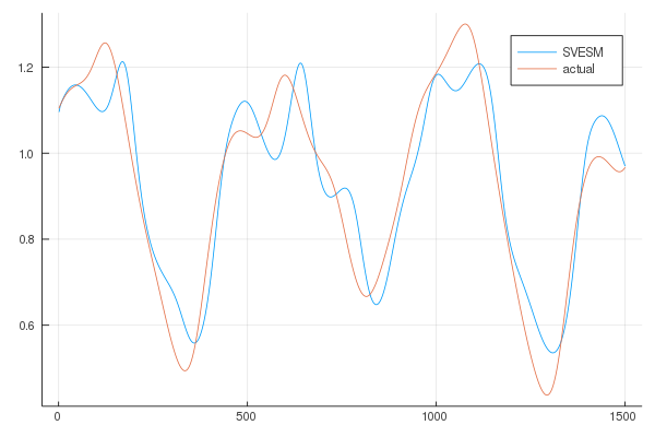
From the results it is clear that the SVESM performs better.
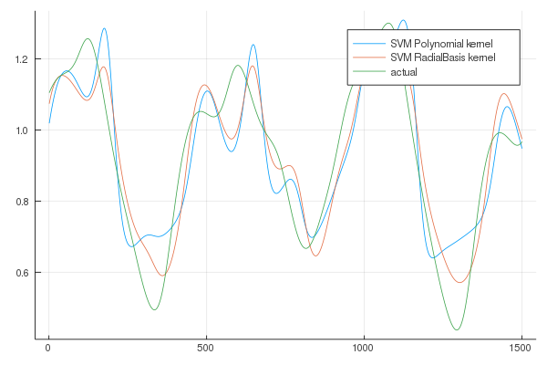
Noisy training and noiseless testing
Adding normally distributed white noise to the training input dataset we obtain the following results for the nmrse:
Training on noisy data and testing on noiseless data...
SVESM nmrse for noisy training and noiseless testing: 0.415
SVM Poly kernel nmrse for noisy training and noiseless testing: 0.643
SVM RadialBasis kernel nmrse for noisy training and noiseless testing: 0.557
The plots are

Also in this case the performance of the SVESM is superior to SVR.
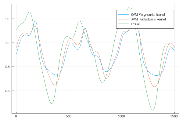
Noisy training and testing
For the last comparison the results are as follows
Training and testing on noisy data...
SVESM nmrse for noisy training and testing: 0.439
SVM Poly kernel nmrse for noisy training and testing: 0.724
SVM RadialBasis kernel nmrse for noisy training and testing: 0.648
And in this case as well the proposed model outperforms SVR.
As always, if you have any questions regarding the model, the package or you have found errors in my post, please don’t hesitate to contact me!
Citing
Part of the work done for this project has been published. If this post or the ReservoirComputing.jl software has been helpful, please consider citing the accompanying paper:
@article{JMLR:v23:22-0611,
  author  = {Francesco Martinuzzi and Chris Rackauckas and Anas Abdelrehim and Miguel D. Mahecha and Karin Mora},
  title   = {ReservoirComputing.jl: An Efficient and Modular Library for Reservoir Computing Models},
  journal = {Journal of Machine Learning Research},
  year    = {2022},
  volume  = {23},
  number  = {288},
  pages   = {1--8},
  url     = {http://jmlr.org/papers/v23/22-0611.html}
}
References
[1] Drucker, Harris, et al. “Support vector regression machines.” Advances in neural information processing systems. 1997.
[2] Smola, Alex J., and Bernhard Schölkopf. “A tutorial on support vector regression.” Statistics and computing 14.3 (2004): 199-222.
[3] VladimirN. Vapnik, The Nature of Statistical Learning Theory, Springer, 1995.
[4] Shi, Zhiwei, and Min Han. “Support vector echo-state machine for chaotic time-series prediction.” IEEE transactions on neural networks 18.2 (2007): 359-372.