Continuing to leverage similarities between Reservoir Computing models and Kernel machines, this week’s implementation merges the Bayesian approach of Gaussian Process Regression (GPR) to the Echo State Networks (ESN). After the usual overview of the theory, a computational example will be shown.
Gaussian Process Regression
The following section is meant as a quick reminder of the deep theory behind Gaussian Processes and its purpose is to illustrate how this approach is a good fit for ESNs. An in depth chapter on GP regression can be found in [1]. A good introduction is also given in the paper that illustrates the implementation of Echo State Gaussian Processes (ESGP) [2]. In this introduction we will heavily follow the second reference, to keep the notation consistent.
A Gaussian Process (GP) is defined as a collection of random variables, any finite of which have a joint Gaussian distribution. A (GP) is completely specified by its mean function and covariance function: $$m(\textbf{x}) = \mathbb{E}[f(\textbf{x})]$$ $$k(\textbf{x}, \textbf{x}’) = \mathbb{E}[(f(\textbf{x})-m(\textbf{x}))(f(\textbf{x}’)-m(\textbf{x}’))] $$ and the GP can be written as $$f(\textbf{x}) \sim GP(m(\textbf{x}), k(\textbf{x}, \textbf{x}’))$$ An usual choice for the mean function is the zero mean function \( m(\textbf{x} = 0) \), and for the covariance function there is a large variety of kernel functions to choose from. In fact there are so many that one can be overwhelmed by the choice; if this is the case, a good introduction and overview can be found in [3].
Given our data, consisting in the samples \( ( (\textbf{x}_i, y_i) | i = 1,…,N ) \), where \( \textbf{x}_i \) is the d-dimensional observation and \( y_i \) is the correleted target values, we want to be able to predict \( y_* \) given \( \textbf{x}_* \). The response variables \( y_i \) are assumed to be dependent on the predictors \( \textbf{x}_i \):
$$y_i \sim \mathcal{N} (f(\textbf{x}_i), \sigma ^2), i=1,…,N$$
Once defined mean and kernel functions one can obtain the predicted mean and variance: $$\mu _* = \textbf{k}(\textbf{x}_*)^T(\textbf{K}(X, X)+\sigma ^2 \textbf{I}_N)^{-1}\textbf{y}$$
$$\sigma ^2 _* = k(\textbf{x}_, \textbf{x} _) - \textbf{k}(\textbf{x}_)^T(\textbf{K}(X, X)+\sigma ^2 \textbf{I}_N)^{-1} \textbf{k}(\textbf{x}_)$$
where \( \textbf{K}(X, X) \) is the matrix of the covariances (design matrix). The optimization of the hyperparameters is usually done by maximization of the model marginal likelihood.
Echo State Gaussian Processes
Using the definition given in the paper [2] an ESGP is a GP the covariance of which is taken as a kernel function over the states of a ESN, postulated to capture the dynamics within a set of sequentially interdependent observations. In this case the feature mapping is explicit, no kernel trick is adopted.
One of the improvements of this approach against strandard linear regression is the possibility to obtain a measure of uncertainty for the obtained predictions. Furthermore, one can consider this a generalization of simple regression: in fact using a simple linear kernel and setting \( \sigma ^2 = 0 \) the results should be the same of those obtained by plain linear regression.
The paper shows results obtained using the Gaussian RBF kernel, but the high number of kernel available and the possibility to use combination of them makes this approach really versatile and, as of now, somewhat understudied.
Implementation in ReservoirComputing.jl
Building on the package GaussianProcesses it was possible to create a ESGPtrain function as well as a ESGPpredict and a ESGPpredict_h_steps function, with a similar behaviour to the ESN counterpart. The ESGPtrain function takes as input:
esn: the previously defined ESN
mean: a GaussianProcesses.Mean struct, to choose between the ones provided by the GaussianProcesses package
kernel: a GaussianProcesses.Kernel struct, to choose between the ones provided by the GaussianProcesses package
lognoise: optional value with default = -2
optimize: optional value with default = false. If = true the hyperparameters are optimized using Optim.jl. Since gradients are available for all mean and kernel functions, gradient based optimization techniques are recommended.
optimizer: optional value with default = Optim.LBFGS()
y_target: optional value with default = esn.train_data. This way the system learns to predict the next step in the time series, but the user is free to set other possibilities.
The function returns a trained GP, that can be used in ESGPpredict or ESGPpredict_h_steps. They both take as input
- esn: the previously defined ESN
- predict_len: number of steps of the prediction
- gp: a trained GaussianProcesses.GPE struct
in addition ESGPpredict_h_steps requires
- h_steps: the h steps ahead in wich the model will run autonomously
- test_data: the testing data, to be given as input to the model every h-th step.
Example
Similarly to last week the example is based on the Mackey Glass system. It can be described by
$$\frac{dx}{dt} = \beta x(t)+\frac{\alpha x(t-\delta)}{1+x(t-\delta)^2}$$
and the values adopted in [2] are
- \(\beta = -0.1 \)
- \(\alpha = 0.2 \)
- \(\delta = 17 \)
- \( dt = 0.1 \)
Furthermore the time series is rescaled in the range \( [-1, 1] \) by application of a tangent hyperbolic transform \( y_{ESN}(\text{t}) = \text{tanh}(\text{y}(t)-1) \). To evaluate the precision of our results we are going to use root mean square deviation (rmse), defined as:
$$\textbf{rmse} = \sqrt{\frac{\sum_{i=1}^{T_n}(y_d(i)-y(i))^2}{T_n}}$$
where
- \(y_d(i) \) is the target value
- \(y(i) \) is the predicted value
- \(T_d \) is the number of test examples
The ESN parameters are as follows
const shift = 100
const train_len = 6000
const test_len =1500

const approx_res_size = 400
const sparsity = 0.1
const activation = tanh
const radius = 0.99
const sigma = 0.1

const alpha = 0.2
const nla_type = NLADefault()
const extended_states = true
Something worth pointing out is that for the first time we have found a value of alpha other than 1: this means we are dealing with a leaky ESN. Following the paper we will try to give a fair comparison between ESN trained with Ridge regression , ESGP and SVESM. Since the parameters for ESN with Ridge and SVESM are missing in the paper, we thought best to use “default” parameters for all the model involved: using optimization only on one model did not seem like a fair comparison. Both in SVESM and ESGP the kernel function used is Gaussian RBF.
The results are as follows:
ESGP RBF rmse: 0.0298
ESN ridge rmse: 0.1718
SVESM RBF rmse: 0.1922
We can clearly see that the proposed model is outperforming the other models proposed. We mentioned that one of the improvements of this models was the measure of uncertainty relative to the prediction. The ESGPpredict function also returns the variance of the prediction, that can be plotted alongside the results:
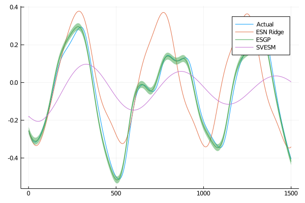
From the plot is even more clear that the ESGP is more capable of reproducing the behaviour of the Mackey-Glass system. Like in the paper the worst performing model for this specific task is the SVESM.
Beside a better analysis of the parameters to use in this case, it would also be interesting to see a comparison between the normal GPR with different kernel functions and the ESGP with the same kernel functions.
As always, if you have any questions regarding the model, the package or you have found errors in my post, please don’t hesitate to contact me!
Citing
Part of the work done for this project has been published. If this post or the ReservoirComputing.jl software has been helpful, please consider citing the accompanying paper:
@article{JMLR:v23:22-0611,
  author  = {Francesco Martinuzzi and Chris Rackauckas and Anas Abdelrehim and Miguel D. Mahecha and Karin Mora},
  title   = {ReservoirComputing.jl: An Efficient and Modular Library for Reservoir Computing Models},
  journal = {Journal of Machine Learning Research},
  year    = {2022},
  volume  = {23},
  number  = {288},
  pages   = {1--8},
  url     = {http://jmlr.org/papers/v23/22-0611.html}
}
Documentation
[1] Rasmussen, Carl Edward. “Gaussian processes in machine learning.” Summer School on Machine Learning. Springer, Berlin, Heidelberg, 2003.
[2] Chatzis, Sotirios P., and Yiannis Demiris. “Echo state Gaussian process.” IEEE Transactions on Neural Networks 22.9 (2011): 1435-1445.