The standard construction of the reservoir matrix $ \textbf{W} $ for Echo State Networks (ESN) is based on initializing $ \textbf{W} $ using specific schemes, usually generating random numbers and then rescaling it to make sure that the spectral radius is less or equal to a chosen number. This procedure is effective, but in literature other ways are explored. In this week we implemented a Singular Value Decomposition (SVD)-based algorithm, described in [1], that is capable of obtaining a sparse matrix suitable for the ESNs. In this post we are going to describe the theory behind the implementation and then a couple of examples will be given.

Singular Value Decomposition reservoir construction

One of the key aspects the an ESN is for its reservoir to posses the Echo State Property (ESP) [2]. A sufficient condition to obtain it is to construct the reservoir with a spectral radius less than 1. While using the architecture explained in the opening ensures this condition, it doesn’t take into account the singular values information of $ \textbf{W} $, and it doesn’t allow much control over the construction of said matrix. An alternative could be to leverage the SVD to build a reservoir matrix given the largest singular value. To fully comprehend this procedure firstly we have to illustrate what SVD consists of.

Let us consider the reservoir matrix $ \textbf{W} \in \mathbb{R}^{N \times N}$; this matrix can be expressed as $ \textbf{W} = \textbf{U}\textbf{S}\textbf{V} $ where $ \textbf{U}, \textbf{V} \in \mathbb{R}^{N \times N}$ are orthogonal matrices and $ \textbf{S}=\text{diag}(\sigma _1, …, \sigma _N) $ is a diagonal matrix whose entries are ordered in increasing order. The values $ \sigma _i $ are called the singular values of $ \textbf{W} $. Given any diagonal matrix $ \textbf{S} $, and orthogonal matrices $ \textbf{U}, \textbf{V} $ the matrix $ \textbf{W} $ obtained as $ \textbf{W} = \textbf{U}\textbf{S}\textbf{V} $ has the same singular values as $ \textbf{S} $.

This method provides an effective way of ensuring the ESP without the scaling of the reservoir weights. Instead of using orthogonal matrices $ \textbf{U}, \textbf{V} $, that could produce a dense matrix $ \textbf{W} $, the authors opted for a two dimensional rotation matrix $ \textbf{Q}(i, j, \theta) \in \mathbb{R}^{N \times N}$ with $ \textbf{Q}_{i,i} = \textbf{Q}_{j,j} = \text{cos}(\theta)$, $ \textbf{Q}_{i,j} = -\text{sin}(\theta)) $, $ \textbf{Q}_{j,i} = \text{sin}(\theta)) $ with $ i, j $ random values in [1, N] and $ \theta $ random value in [-1, 1]. The algorithm proposed is as follows:

Choose a predefined $ \sigma _N $ in the range [0, 1] and generate $ \sigma _i, i=1,…, N-1 $ in the range (0, $ \sigma _N $]. This values are used to create a diagonal matrix $ \textbf{S}=\text{diag}(\sigma _1, …, \sigma _N) $. With $ h=1 $ let $ \textbf{W}_1 = \textbf{S} $.
For $ h = h + 1 $ randomly choose the two dimensional matrix $ \textbf{Q}(i, j, \theta) $ as defined above. $ \textbf{W} _h = \textbf{W} _{h-1} \textbf{Q}(i, j, \theta)$ gives the matrix $ \textbf{W} $ for the step $ h $. This procedure is repeated until the chosen density is reached.

Implementation in ReservoirComputing.jl

The implementation into code is extremely straightforwad: following the instructions in the paper a function pseudoSVD is created which takes as input the following

dim: the desired dimension of the reservoir
max_value: the value of the largest of the singular values
sparsity: the sparsity for the reservoir
sorted: optional value. If = true (default) the singular values in the diagonal matrix will be sorted.
reverse_sort: optional value if sort = true. If = true (default = false) the singular values in the diagonal matrix will be sorted in a decreasing order.

Examples

Original ESN

Testing the SVD construction on the original ESN we can try to reproduce the Lorenz attractor, with similar parameters as given in the Introduction to Reservoir Computing

approx_res_size = 300
radius = 1.2
sparsity = 0.1
max_value = 1.2
activation = tanh
sigma = 0.1
beta = 0.0
alpha = 1.0
nla_type = NLADefault()
extended_states = false

The values of the largest singular value for the construction of the SVD based reservoir is equal to the spectral radius of the standard reservoir, that in this case is greater than one. A plot of the results shows:

lorenz_coord

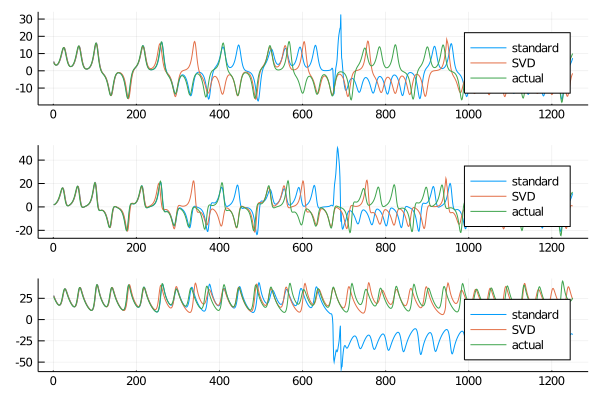
This construction is capable of reproducing the Lorenz system in the short term, and behaves better in the long term than the standard implementation, or at least in this example it does. A more in depth analysis is needed for the consistency of the results and the behavior of the SVD reservoir when the largest singular value is set greater than one and when one of the non linear algorithms is applied.

Ridge ESN, SVESM and ESGP

In order to test this implementation for others ESN architectures currently implemented in ReservoirComputing.jl we choose to use the same examples as last week, based on the Mackey-Glass system:

$$\frac{dx}{dt} = \beta x(t)+\frac{\alpha x(t-\delta)}{1+x(t-\delta)^2}$$

with the same values:

$\beta = -0.1 $
$\alpha = 0.2 $
$\delta = 17 $
$ dt = 0.1 $

Furthermore the time series is rescaled in the range $ [-1, 1] $ by application of a tangent hyperbolic transform $ y_{ESN}(\text{t}) = \text{tanh}(\text{y}(t)-1) $. To evaluate the precision of our results we are going to use root mean square deviation (rmse), defined as:

$$\textbf{rmse} = \sqrt{\frac{\sum_{i=1}^{T_n}(y_d(i)-y(i))^2}{T_n}}$$

where

$y_d(i) $ is the target value
$y(i) $ is the predicted value
$T_d $ is the number of test examples

The ESN parameters are as follows

const shift = 100
const train_len = 6000
const test_len =1500

const approx_res_size = 400
const sparsity = 0.1
const activation = tanh
const radius = 0.99
const max_value = 0.99
const sigma = 0.1

const alpha = 0.2
const nla_type = NLADefault()
const extended_states = true

The largest singular value was set equal to the spectral radius for the standard construction. Averaging on ten runs the results are as follows:

rmse ESGP:
Classic reservoir: 0.077
SVD reservoir: 0.205
rmse ridge ESN:
Classic reservoir: 0.143
SVD reservoir: 0.146
rmse SVESM:
Classic reservoir: 0.232
SVD reservoir: 0.245

For the ESGP this procedure yields far worst performances than the standard counterpart. For the ridge ESN and SVESM the results are almost identical.

The results obtained are interesting and for sure more testing is needed. Some sperimentation on the h steps ahead prediction could be done, as well as giving different values for the spectral radius and largest singular value, since in all the examples examined the spectral radius was chosen following the literature, and hence could be more optimized that the largest values that we used.

Citing

Part of the work done for this project has been published. If this post or the ReservoirComputing.jl software has been helpful, please consider citing the accompanying paper:

@article{JMLR:v23:22-0611,
  author  = {Francesco Martinuzzi and Chris Rackauckas and Anas Abdelrehim and Miguel D. Mahecha and Karin Mora},
  title   = {ReservoirComputing.jl: An Efficient and Modular Library for Reservoir Computing Models},
  journal = {Journal of Machine Learning Research},
  year    = {2022},
  volume  = {23},
  number  = {288},
  pages   = {1--8},
  url     = {http://jmlr.org/papers/v23/22-0611.html}
}

Documentation

[1] Yang, Cuili, et al. “Design of polynomial echo state networks for time series prediction.” Neurocomputing 290 (2018): 148-160.

[2] Jaeger, Herbert. “The “echo state” approach to analysing and training recurrent neural networks-with an erratum note.” Bonn, Germany: German National Research Center for Information Technology GMD Technical Report 148.34 (2001): 13.

Singular Value Decomposition reservoir construction#

Implementation in ReservoirComputing.jl#

Examples#

Original ESN#

Ridge ESN, SVESM and ESGP#

Citing#

Documentation#