This post is meant to be a high level comparison of different variations of the Echo State Network (ESN) model, implemented in the first month of Google Summer of Code. The theoretical background for all the proposed models has already been covered in past posts, so we will not touch on it in this one to keep things as thight as possible; if one is interested all my previous posts can be found here. The ESNs are known for their capability of yielding good short term predictions and long term reconstructions of chaotic systems: in order to prove this we are going to test all the proposed models using the Lorenz system.
In order to determine the accuracy of the results we will use two different methods:
- For the short term accuracy we chose an arbitrary time horizon and the difference between the actual timeseries, obtained solving the differential equations of the Lorenz system, and the predicted timeseries will be evaluated using the Root Mean Square Deviation (RMSE). The rmse implementation in Julia is done with the following function
function rmse(y, yt)
    rmse = 0.0
    for i=1:size(y, 1)
        rmse += (y[i]-yt[i])^2.0
    end
    rmse = sqrt(rmse/(size(y, 1)))
    return rmse
end
- For the long term climate we chose to follow the approach of Pathak [1] and we will show the return map of successive maxima of \( z(t) \). To get this data we leveraged the function
findlocalmaximaof the package Images.jl. The Julia function used to get the vector of local maxima is defined as follows
using Images
function local_maxima(input_data)
    maxs_cart = findlocalmaxima(input_data)
    maxs = [idx[1] for idx in maxs_cart]
    max_values = []
    for max in maxs
        push!(max_values, input_data[max])
    end
    return max_values
end
The data used for all the training and prediction for the ESN in this work is obtained in the following way:
u0 = [1.0,0.0,0.0]
tspan = (0.0,2000.0)
p = [10.0,28.0,8/3]
#define lorenz system
function lorenz(du,u,p,t)
    du[1] = p[1]*(u[2]-u[1])
    du[2] = u[1]*(p[2]-u[3]) - u[2]
    du[3] = u[1]*u[2] - p[3]*u[3]
end
#solve and take data
prob = ODEProblem(lorenz, u0, tspan, p)
sol = solve(prob, RK4(), adaptive=false, dt=0.02)
v = sol.u
data = Matrix(hcat(v...))
shift = 300
train_len = 5000
predict_len = 1250
return_map_size = 20000
train = data[:, shift:shift+train_len-1]
test = data[:, shift+train_len:shift+train_len+predict_len-1]
return_map = data[:,shift+train_len:shift+train_len+return_map_size-1];
Where the test data will be used for display and the first 400 timesteps for the short term prediction. The return_map data will instead be used for the creation of the return maps.
Ordinary ESN
The Ordinary Least Squares (OLS) trained ESN is the model used in [1] to accurately predict the Lorenz system in the short term and replicate its climate in the long term. We will use the same construction given in their paper, and most of these parameters will be used also for the other variation presented in this post. The parameters and the training for the ESN are as follows
using ReservoirComputing
using Random

approx_res_size = 300
radius = 1.2
degree = 6
activation = tanh
sigma = 0.1
beta = 0.0
alpha = 1.0
nla_type = NLAT2()
extended_states = false

Random.seed!(4242)
esn = ESN(approx_res_size, train, degree, radius,
    activation = activation, alpha = alpha, sigma = sigma, nla_type = nla_type, extended_states = extended_states)
@time W_out = ESNtrain(esn, beta)
output = ESNpredict(esn, predict_len, W_out)
1.963047 seconds (5.79 M allocations: 310.671 MiB, 4.29% gc time)
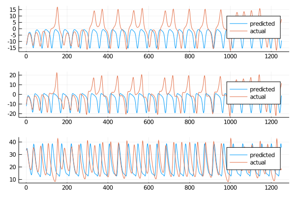
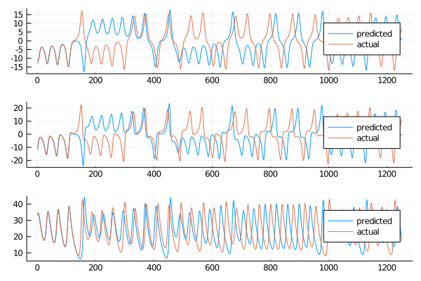
We can plot a comparison to have a visual feedback for the coordinates
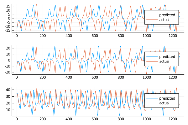
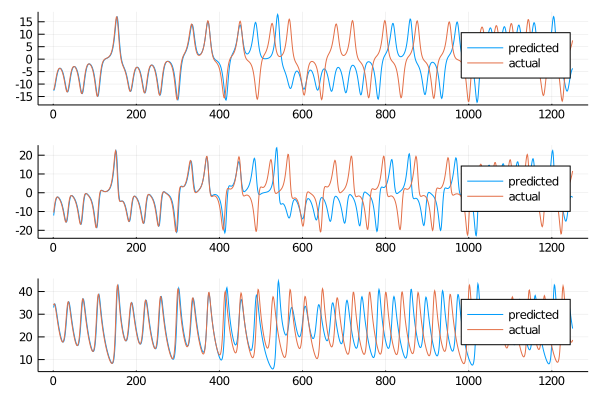
plot(transpose(output),layout=(3,1), label="predicted")
plot!(transpose(test),layout=(3,1), label="actual")
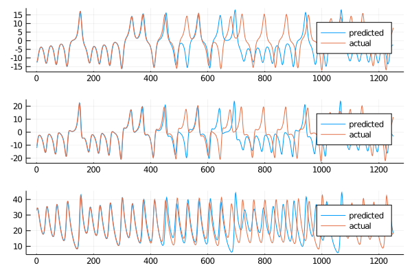 From just a quick eye test we can see that the short term prediction is rather good, and in the long term the behaviour seems to be in line with the numerical solution. For the short term prediction we are going to use the already defined
 rmse function an all three the variables to check the accuracy. The arbitrary length of the short time horizon is set to 400 and will stay the same all throughout this work.
for i=1:size(data, 1)
    println(rmse(test[i,1:400], output[i, 1:400]))
end
0.9484793317137318
1.4450094312490096
1.769172087306121
Since the values are the lower the better we can be satisfied with what we obtained. This numbers will mostly be used for comparisons between models and their significance by themselves is very limited, also because this is the result of a single run. To show model consistency a more deep analisys has to be conducted, but aslo this aspect will be discussed in the ending section.
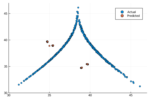
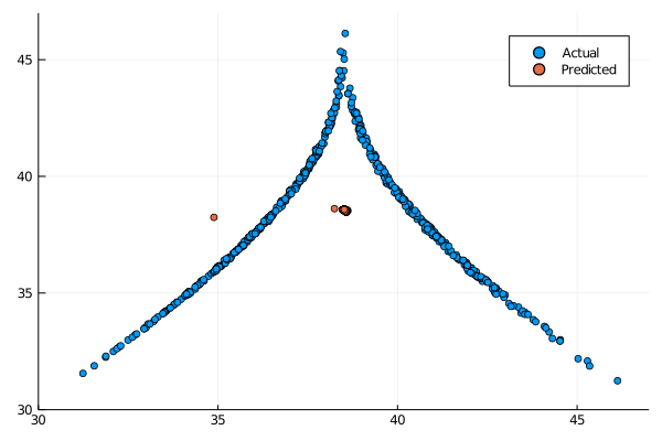
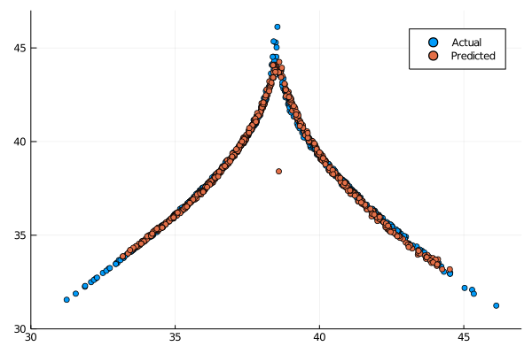
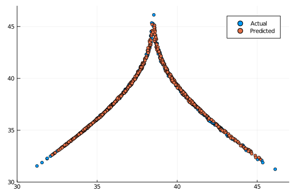
To have quantitative confirmation that our models is capable of predicting a reliable synthetic dataset we are going to predict the system using the return_map dataset, and then plot the consecutives maxima of the \( z(t) \) coordinate.
output_map = ESNpredict(esn, return_map_size, W_out)
max_esn = local_maxima(output_map[3,:])
max_ode = local_maxima(return_map[3,:])
scatter(max_ode[1:end-1], max_ode[2:end], label="Actual")
scatter!(max_esn[1:end-1], max_esn[2:end], label="Predicted")
xlims!((30, 47))
ylims!(30, 47)
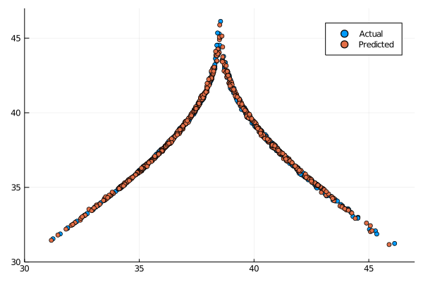
It is nice to see that our results are in line with what is displayed in the paper [2].
Ridge ESN
One usual problem that can be encountered when dealing with OLS is the insurgence of numerical instabilities when inverting \( (\textbf{X} \textbf{X}^T) \) [2] where \( \textbf{X} \) is the feature matrix (states matrix in the case of ESNs). A solution to this is to apply a regularization to the loss function, and one of the most common is the \( L_2 \) regularization. This way we obtain what is called ridge regression or Tikhonov regularization. The ridge ESN is trained in an equal manner as the OLS ESN we discussed above, only setting a parameter beta different than zero. The parameter that we chose is by no mean optimized and it is chosen by manual search, and this holds sadly for all the parameters in the models here presented. In the Conclusions section we will talk a little more about this aspect of this work.
approx_res_size = 300
radius = 1.2
degree = 6
activation = tanh
sigma = 0.1
beta = 0.001
alpha = 1.0
nla_type = NLAT2()
extended_states = false

Random.seed!(4242)
esn = ESN(approx_res_size, train, degree, radius,
    activation = activation, alpha = alpha, sigma = sigma, nla_type = nla_type, extended_states = extended_states)
@time W_out = ESNtrain(esn, beta)
output = ESNpredict(esn, predict_len, W_out);
2.223003 seconds (5.79 M allocations: 310.671 MiB, 2.85% gc time)
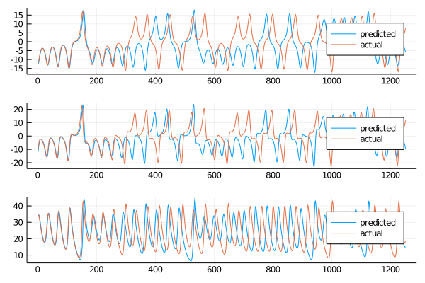
This methods is just a little slower, as it has to be expected. It is still an acceptable by any means. Plotting the results we obtain:
plot(transpose(output),layout=(3,1), label="predicted")
plot!(transpose(test),layout=(3,1), label="actual")
 The behaviour is similar to the standard ESN, but let’s take a look at the short and long term.
for i=1:size(data, 1)
    println(rmse(test[i,1:400], output[i, 1:400]))
end
5.3658081215986
6.552586461430827
4.995926155420491
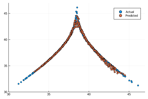
It was clearly visible before that the short term behaviour was not as good as the standard counterpart. The long term predictions are still acceptable, as we can see here:
output_map = ESNpredict(esn, return_map_size, W_out)
max_esn = local_maxima(output_map[3,:])
max_ode = local_maxima(return_map[3,:])
scatter(max_ode[1:end-1], max_ode[2:end], label="Actual")
scatter!(max_esn[1:end-1], max_esn[2:end], label="Predicted")
xlims!((30, 47))
ylims!(30, 47)
Clearly in this case the original architecture proves superior in the short term, but in the long term the both are really viable. Depending on the situation and dataset the ridge ESN can be a valide choice for accuracy and speed of training, and it could also be the only viable choice between the two, if the problem is ill-posed.
Lasso ESN
Another common regularization for the OLS regression is the \( L_1 \) regularization, resulting in a regression model called Lasso. This is a stronger regularization, and it shows from the results. The ESN is built in the same way as before, only this time the parameter beta indicates the Lasso regularizer. Since the expression doesn’t have a closed form solution we will need a different solver, in this case ProxGrad. For this we will need to import a different package, called MLJLinearModels.jl.
using MLJLinearModels
approx_res_size = 300
radius = 1.2
degree = 6
activation = tanh
sigma = 0.1
beta = 1*10^(-7)
alpha = 1.0
nla_type = NLAT2()
extended_states = false

Random.seed!(4242)
esn = ESN(approx_res_size, train, degree, radius,
    activation = activation, alpha = alpha, sigma = sigma, nla_type = nla_type, extended_states = extended_states)
@time W_out = ESNtrain(Lasso(beta, ProxGrad(max_iter=10000)), esn)
output = ESNpredict(esn, predict_len, W_out)
24.400234 seconds (9.82 M allocations: 1.534 GiB, 1.17% gc time)
The training time is slower than the couple of models we showed before. This difference is mainly to the already mentioned lack of closed form solution for the Lasso regression. Let us plot the results to start the analysis the results.
plot(transpose(output),layout=(3,1), label="predicted")
plot!(transpose(test),layout=(3,1), label="actual")
 It is clear that this regularization is not capable of returning an accurate prediction, both short term and long term. Let’s print the rmse
for i=1:size(data, 1)
    println(rmse(test[i,1:400], output[i, 1:400]))
end
11.769042467212172
13.599065187854675
10.651859641213985
and plot the return map
output_map = ESNpredict(esn, return_map_size, W_out)
max_esn = local_maxima(output_map[3,:])
max_ode = local_maxima(return_map[3,:])
scatter(max_ode[1:end-1], max_ode[2:end], label="Actual")
scatter!(max_esn[1:end-1], max_esn[2:end], label="Predicted")
xlims!((30, 47))
ylims!(30, 47)
From this results is clear that the \( L_1 \) regularization is not capable of good short term prediction and in the long term yields a periodic timeseries, as we can see from the return map, only showing values in 5 contained regions.
Huber loss function
Not only the squared function can be used as a loss function: in literature it has also been proposed the use of the Huber loss function, supposedly more strong in the presence of outliers. The dataset we are using is free of them, but this function should still be able to give accurate results. Since we can apply regularization also in this case, we are going to explore the two cases already explored for the squared function: \( L_2 \) regularization and \( L_1 \) regularization.
\( L_2 \) Normalization
Again leveraging the MLJLinearModels package we can construct our ESN
approx_res_size = 300
radius = 1.2
degree = 6
activation = tanh
sigma = 0.1
beta = 0.001
alpha = 1.0
nla_type = NLAT2()
extended_states = false

Random.seed!(4242)
esn = ESN(approx_res_size, train, degree, radius,
    activation = activation, alpha = alpha, sigma = sigma, nla_type = nla_type, extended_states = extended_states)
@time W_out = ESNtrain(RobustHuber(0.5, beta, 0.0, Newton()), esn)
output = ESNpredict(esn, predict_len, W_out)
9.397286 seconds (14.37 M allocations: 1.748 GiB, 2.88% gc time)
The training time is less than the Lasso regularization, but more than the OLS and Ridge training. Plotting the data we obtain:
plot(transpose(output),layout=(3,1), label="predicted")
plot!(transpose(test),layout=(3,1), label="actual")
Let’s go explore the rmse for the short term:
for i=1:size(data, 1)
    println(rmse(test[i,1:400], output[i, 1:400]))
end
5.36580225918975
6.552573774882654
4.995989255679152
The results seem similar to the Ridge ESN. For the long term the return map shows the following:
output_map = ESNpredict(esn, return_map_size, W_out)
max_esn = local_maxima(output_map[3,:])
max_ode = local_maxima(return_map[3,:])
scatter(max_ode[1:end-1], max_ode[2:end], label="Actual")
scatter!(max_esn[1:end-1], max_esn[2:end], label="Predicted")
xlims!((30, 47))
ylims!(30, 47)
Even though they are not as clear cut as the OLS ESN and Ridge ESN the long term behaviour is still acceptable.
\( L_1 \) Normalization
Since the Lasso ESN showed the worst results of all the model seen until now this could indicate that the \( L_1 \) norm is not suited for this task. To have confirmation of this intuition we can train the Huber ESN with the \( L_1 \) norm to see if it yields better results than the Lasso ESN.
approx_res_size = 300
radius = 1.2
degree = 6
activation = tanh
sigma = 0.1
beta = 1*10^(-7)
alpha = 1.0
nla_type = NLAT2()
extended_states = false

Random.seed!(4242)
esn = ESN(approx_res_size, train, degree, radius,
    activation = activation, alpha = alpha, sigma = sigma, nla_type = nla_type, extended_states = extended_states)
@time W_out = ESNtrain(RobustHuber(0.5, 0.0, beta, ProxGrad(max_iter=10000)), esn)
output = ESNpredict(esn, predict_len, W_out)
30.699361 seconds (12.60 M allocations: 3.398 GiB, 1.40% gc time)
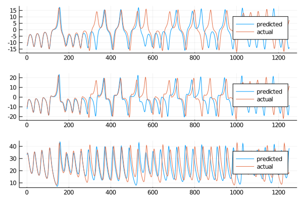
As expected the training time is in line with the Lasso ESN. Plotting the results we can see that sadly they are worst than the Lasso counterpart
plot(transpose(output),layout=(3,1), label="predicted")
plot!(transpose(test),layout=(3,1), label="actual")
Calculating the rmse for the first 400 steps returns
for i=1:size(data, 1)
    println(rmse(test[i,1:400], output[i, 1:400]))
end
8.247263444106135
9.896322405158461
12.569601968865513
And the return map clearly shows a periodic long term behaviour:
output_map = ESNpredict(esn, return_map_size, W_out)
max_esn = local_maxima(output_map[3,:])
max_ode = local_maxima(return_map[3,:])
scatter(max_ode[1:end-1], max_ode[2:end], label="Actual")
scatter!(max_esn[1:end-1], max_esn[2:end], label="Predicted")
xlims!((30, 47))
ylims!(30, 47)
The periodicity is more pronounced than the Lasso ESN, making this model the worst performing so far on this task.
Different reservoir construction
For all the model proposed we used the standard construction of the reservoir, based on the rescaling of the spectral radius to be less than a given value. In literature there are other alternatives explored and in the ReservoirComputing.jl package is present the implementation of an algorithm for the construction of the reservoir matrix based on the Single Value Decomposition (SVD), proposed in [4]. We are going to give the results using this construction only for the OLS ESN, but a more wide study could be done comparing the performances of all the proposed models using the two different implementations of the reservoir.
approx_res_size = 300
max_value = 1.2
sparsity = 0.1
activation = tanh
sigma = 0.1
beta = 0.0
alpha = 1.0
nla_type = NLAT2()
extended_states = false

Random.seed!(4242)
W_in = init_dense_input_layer(approx_res_size, size(train, 1), sigma)
W_new = pseudoSVD(approx_res_size, max_value, sparsity, reverse_sort = true)
esn = ESN(W_new, train, W_in,
    activation = activation, alpha = alpha, nla_type = nla_type, extended_states = extended_states)
@time W_out = ESNtrain(esn, beta)
output = ESNpredict(esn, predict_len, W_out)
0.994207 seconds (3.18 M allocations: 188.436 MiB, 3.64% gc time)
The training time is as fast as the normal OLS ESN, as it is to be expected. Plotting the result we obtain
plot(transpose(output),layout=(3,1), label="predicted")
plot!(transpose(test),layout=(3,1), label="actual")
 From the plot it seems that the model is producing an acceptable Lorenz system surrogate dataset. The short term will not be the best but in the long term maybe the model could behave as the OLS ESN.
for i=1:size(data, 1)
    println(rmse(test[i,1:400], output[i, 1:400]))
end
8.299351042330624
9.954728072605832
9.507147274321735
Not as good as the normal reservoir counterpart, but let’s look at the return map for the long term behaviour:
output_map = ESNpredict(esn, return_map_size, W_out)
max_esn = local_maxima(output_map[3,:])
max_ode = local_maxima(return_map[3,:])
scatter(max_ode[1:end-1], max_ode[2:end], label="Actual")
scatter!(max_esn[1:end-1], max_esn[2:end], label="Predicted")
xlims!((30, 47))
ylims!(30, 47)
Event though it seemed that the predicted coordinates had a similar behaviour as the actual Lorenz system the return map clearly shows that in the long term the behaviour is not consistent. This approach to reservoir construction is of course pretty novel and has to pass several optimization steps for its parameters in order to be production ready, but this first test is somewhat disappointing.
Echo State Gaussian Processes
Firstly proposed in [3] the Echo State Gaussian Processes (ESGP) can be considered an extension of the ESN. In the original paper only the Radial Basis function is explored for the prediction, but in this post we wanted to give a couple of examples of others kernels, so we will use also the Matern kernel and the Polynomial kernel for the prediction of the Lorenz system. The construction of this model is based on GaussianProcesses, so in the first run we will need to import that package as well.
Radial Basis kernel
Starting from the kernel used in the original paper, we also set the non linear algorithm to the default one, equal to none. The behaviour with different algorithms for this family of models has not been investigated and could be subject of future works, but for now we will just limit the work to the standard one. Keeping the other parameters equal the ESGP can be built in the following way
using GaussianProcesses
#model parameters
degree = 6
approx_res_size = 300
radius = 1.2
activation = tanh
sigma = 0.1
alpha = 1.0
nla_type = NLADefault()
extended_states = false

#create echo state network
Random.seed!(4242)
esn = ESN(approx_res_size, train, degree, radius,
    activation = activation, alpha = alpha, sigma = sigma, nla_type = nla_type, extended_states = extended_states)

mean = MeanZero()
kernel = SE(1.0, 1.0)
@time gp = ESGPtrain(esn, mean, kernel, lognoise = -2.0, optimize = false);
output, sigmas = ESGPpredict(esn, predict_len, gp)
43.323255 seconds (6.81 M allocations: 2.053 GiB, 2.53% gc time)
The slowest time so far, but maybe the results will be worth the extra seconds it took to train
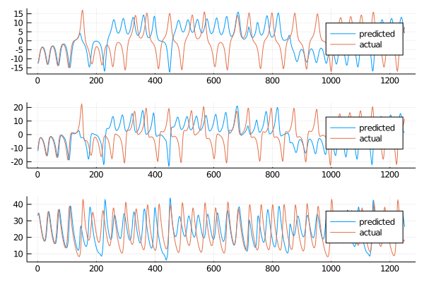
plot(transpose(output),layout=(3,1), label="predicted")
plot!(transpose(test),layout=(3,1), label="actual")
 The results do not look bad, in the short term sadly emerges a discrepancy early on that will lower the rmse values
for i=1:size(data, 1)
    println(rmse(test[i,1:400], output[i, 1:400]))
end
10.5883475480527
11.759694995689005
6.745353916847517
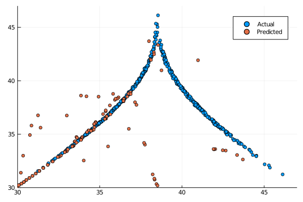
As expected the rmses are not the greatest, but the model can still recover with a nice display of long term behaviour
output_map, sigma_map = ESGPpredict(esn, return_map_size, gp)
max_esn = local_maxima(output_map[3,:])
max_ode = local_maxima(return_map[3,:])
scatter(max_ode[1:end-1], max_ode[2:end], label="Actual")
scatter!(max_esn[1:end-1], max_esn[2:end], label="Predicted")
xlims!((30, 47))
ylims!(30, 47)
and indeed it does, outside of a single point in a strange location the model seems to capture the Lorenz climate quite well, not quite as good as the OLS ESN or even the Ridge ESN.
Matern kernel
Another common kernel is the Matern kernel, and training the ESGP using this kernel is a straightforward process, identical to the one we just followed for the Radial Basis kernel:
#model parameters
degree = 6
approx_res_size = 300
radius = 1.2
activation = tanh
sigma = 0.1
alpha = 1.0
nla_type = NLADefault()
extended_states = false

#create echo state network
Random.seed!(4242)
esn = ESN(approx_res_size, train, degree, radius,
    activation = activation, alpha = alpha, sigma = sigma, nla_type = nla_type, extended_states = extended_states)

mean = MeanZero()
kernel = Matern(1/2, 1.0, 1.0)
@time gp = ESGPtrain(esn, mean, kernel, lognoise = -2.0, optimize = false);
output, sigmas = ESGPpredict(esn, predict_len, gp)
40.309179 seconds (1.08 M allocations: 1.761 GiB, 7.58% gc time)
Plotting the results
plot(transpose(output),layout=(3,1), label="predicted")
plot!(transpose(test),layout=(3,1), label="actual")
 The results seem similar to the ones obtained using the Radial Basis kernel. To be sure of this we need to calculate the rmse
for i=1:size(data, 1)
    println(rmse(test[i,1:400], output[i, 1:400]))
end
7.150484170664864
8.520570924338477
7.037257939507858
The lower rmses shows a better short term prediction. Plotting the return map to analize the long term results
output_map, sigma_map = ESGPpredict(esn, return_map_size, gp)
max_esn = local_maxima(output_map[3,:])
max_ode = local_maxima(return_map[3,:])
scatter(max_ode[1:end-1], max_ode[2:end], label="Actual")
scatter!(max_esn[1:end-1], max_esn[2:end], label="Predicted")
xlims!((30, 47))
ylims!(30, 47)
 The return map is not a clear cut as we saw in other models, but for the majority of the times it seems that the model is still capable of retaining the climate of the Lorenz system.
Polynomial kernel
The last kernel for the ESGP is the Polynomial kernel. We are now familiar with the construction
#model parameters
degree = 6
approx_res_size = 300
radius = 1.2
activation = tanh
sigma = 0.1
alpha = 1.0
nla_type = NLADefault()
extended_states = false

#create echo state network
Random.seed!(4242)
esn = ESN(approx_res_size, train, degree, radius,
    activation = activation, alpha = alpha, sigma = sigma, nla_type = nla_type, extended_states = extended_states)

mean = MeanZero()
kernel = Poly(1.0, 1.0, 2)
@time gp = ESGPtrain(esn, mean, kernel, lognoise = -2.0, optimize = false);
output, sigmas = ESGPpredict(esn, predict_len, gp)
16.979100 seconds (4.27 M allocations: 3.025 GiB, 10.13% gc time)
Plotting the results
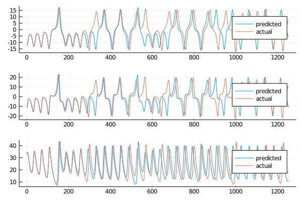
plot(transpose(output),layout=(3,1), label="predicted")
plot!(transpose(test),layout=(3,1), label="actual")
 we can see a nice prediction on the short term. Using once again the rmse
for i=1:size(data, 1)
    println(rmse(test[i,1:400], output[i, 1:400]))
end
0.9128150765679983
1.3969462542792563
1.6437787377104938
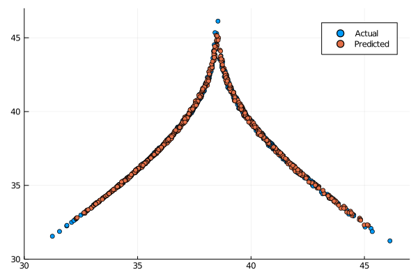
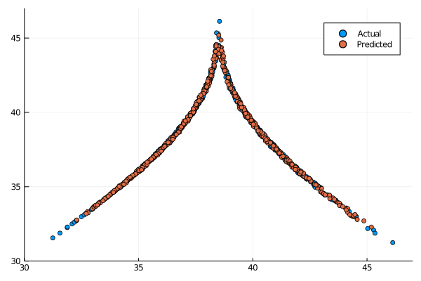
The short term rmse are the best out of the ESGP kernel used until now. Taking a look also to the long term we can see the following
output_map, sigma_map = ESGPpredict(esn, return_map_size, gp)
max_esn = local_maxima(output_map[3,:])
max_ode = local_maxima(return_map[3,:])
scatter(max_ode[1:end-1], max_ode[2:end], label="Actual")
scatter!(max_esn[1:end-1], max_esn[2:end], label="Predicted")
xlims!((30, 47))
ylims!(30, 47)
The results are in line with the OLS ESN. Considering that the results of the OLS ESN were obtained following a published paper and underwent major optimization while the parameters we have chosen are the fruit of a quick manul search we can say that this model could outperform the ESN for chaotic time series prediction.
Conclusions
This post is just scratching the surface on the studies needed for this family of models. As we mentioned numerous times throughout the post, the parameter optimization that was done for this wark was just acceptable, being a manual search starting from values optimized for a specific model (OLS ESN). This fact was most evident when testing the SVD based reservoir construction: even though it is a very similar resulting matrix the results were suboptimal. This could have been just an error in the selection of the parameters, and with a more suiting set this construction could perform as well as the standard one.
But even with more carefully chosen parameters it is necessary to do multiple runs and obtain a large pool of statistics in order to label a model variation more efficient than the other: in this post we have seen that the Polynomial ESGP has returned amazing results, but changing the seed and using a different reservoir the best model could very well be the radial basis ESGP, or the Huber ESN. This work was based on the single run of all the models because is more intended to be a showcase of the new implementations done for the GSoC project, and the reproducibility was the most important aspect of it.
Sadly in this post we weren’t able to showcase the Support Vector Echo State Machines (SVESMs) but the results they obtained wasn’t in line with any of the proposed models, and it performed way worst than even the \( L_1 \) trained ESNs. The paper proposing the models leveraged it to solve a different family of problems, so it could be that this task is not suited for this particular variation of the ESN.
Regarding the ESGP the possible directions for future studies are really numerous: there are a vast number of other avaiable kernels that we didn’t explore, and even in the one we used the possibility to optimize the parameter is built in in the model, and in our case wasn’t used just for time limitations. Not only it is possible to obtain better results that the one we showed purely by parameter optimization but also by using different kernels at the same time: in the Gaussian Processes is usual to see different kernels combined togheter, through multiplication and addition. This possibility adds an incredible perspective to this model, and I hope future studies will takle it.
As usual thanks for reading, if you spot any mistake or are just curious about the model and implementation don’t hesitate to contact me.
Citing
Part of the work done for this project has been published. If this post or the ReservoirComputing.jl software has been helpful, please consider citing the accompanying paper:
@article{JMLR:v23:22-0611,
  author  = {Francesco Martinuzzi and Chris Rackauckas and Anas Abdelrehim and Miguel D. Mahecha and Karin Mora},
  title   = {ReservoirComputing.jl: An Efficient and Modular Library for Reservoir Computing Models},
  journal = {Journal of Machine Learning Research},
  year    = {2022},
  volume  = {23},
  number  = {288},
  pages   = {1--8},
  url     = {http://jmlr.org/papers/v23/22-0611.html}
}
Documentation
[1] Pathak, Jaideep, et al. “Using machine learning to replicate chaotic attractors and calculate Lyapunov exponents from data.” Chaos: An Interdisciplinary Journal of Nonlinear Science 27.12 (2017): 121102.
[2] Lukoševičius, Mantas. “A practical guide to applying echo state networks.” Neural networks: Tricks of the trade. Springer, Berlin, Heidelberg, 2012. 659-686.
[3] Chatzis, Sotirios P., and Yiannis Demiris. “Echo state Gaussian process.” IEEE Transactions on Neural Networks 22.9 (2011): 1435-1445.
[4] Yang, Cuili, et al. “Design of polynomial echo state networks for time series prediction.” Neurocomputing 290 (2018): 148-160.