Up until now we used reservoir generated mainly through a random process, and this approach requires a lot of fine parameter tuning. And even when the optimal parameters are found, the prediction is run-dependent and can show different results with different generations of the reservoir. Is this the only way possible to contruct an Echo State Network (ESN)? Is there a deterministic way to build a ESN? These are the question posed in [1], and the following post is an illustration of the implementation in ReservoirComputing.jl of their construction of a deterministic input layer and three reservoirs. As always we will quickly lay out the theory, then an example will be given.

Minimum complexity reservoir and input layer

The usual construction of a reservoir implies the creation of a random sparse matrix, with given sparsity and dimension, and following rescaling of the values in order to have set the spectral radius to be under a determined value, usually one, in order to ensure the Echo State Property (ESP) [2]. As already stated in the work done in the 4th week, this construction, although efficient, could have some downsides. The particular problem we want to solve with the current implementation is the one given by the randomness of the process: both the reservoir and the input layer construction are initially generated as random and later rescaled. The paper we are following for a possible solution [1] introduces three different constructions for a deterministic reservoir:

Delay Line Reservoir (DLR): is composed of units organized in a line. The elements of the lower subdiagonal of the reservoir matrix have non-zero values, and all are the same.
DLR with backward connections (DLRB): based on the DLR each reservoir unit is also connected to the preceding neuron. This is obtained setting as non-zero the elements of both the upper and lower subdiagonal, with two different values.
Simple Cycle Reservoir (SCR): is composed by units organized in a cycle. The non-zero elements of the reservoir are the lower subdiagonal and the upper right corner, all set to the same weight.

In addition to these reservoirs, also a contruction for the input layer is given: all input connections have the same absolute weight and the sign of each value is determined randomly by a draw from a Bernoulli distribution of mean 1/2. In the paper is stated that any other imposition of sign over the input weight deteriorates the results, so a little randomness is manteined even in this construction, but of course is still far from the original implementation.

Implementation in ReservoirComputing

The implementation of the construction of reservoir and input layer as described in the paper is straightforward: following the instructions we created three different functions for the reservoir named DLR(), DLRB() and SCR() that take as input

res_size the size of the reservoir
weight the value for the weights
fb_weight the value for the feedback weights, only needed for the DLRB() function.

The result of each function is a reservoir matrix with the requested construction. In addition we also added a min_complex_input function, taking as input

res_size the size of the reservoir
in_size the size of the input array
weight the value of the weights

and giving as output the minimum complexity input layer.

Example

For this example we are goind to use the Henon map, defined as $$x_{x+1} = 1 - ax_n^2 + y_n$$ $$ y_{n+1} = bx_n $$

The attractor depends on the two values $ a, b $ and shows chaotic behaviour for the classical values of $ a=1.4 $ and $ b=0.3 $.

To obtain a dataset for the Henon map this time we will use the DynamicalSystems package. Before starting the work we will need to download all the necessary utilies and import them:

using Pkg
Pkg.add("ReservoirComputing")
Pkg.add("Plots")
Pkg.add("DynamicalSystems")
Pkg.add("Statistics")
Pkg.add("LinearAlgebra")
Pkg.add("Random")

using ReservoirComputing
using Plots
using DynamicalSystems
using Statistics
using LinearAlgebra
using Random

Now we can generate the Henon map, which will be shifted by -0.5 and scaled by 2, in order to have consistency with the paper. At the same time we are going to wash out any initial transient and construct the training, train, and testing, test, datasets, following the values given by the paper:

ds = Systems.henon()
traj = trajectory(ds, 7000)
data = Matrix(traj)'

data = (data .-0.5) .* 2
shift = 200
train_len = 2000
predict_len = 3000
train = data[:, shift:shift+train_len-1]
test = data[:, shift+train_len:shift+train_len+predict_len-1]

One step ahead prediction

Now we can set the parameters for the construction of the ESN, for which we followed closely the ones given in the paper, outside for the ridge regression value. Note that since some values are corresponding to our default (activation function, alpha and non linear algorithm) we will omit them for clarity.

approx_res_size = 100
radius = 0.3
sparsity = 0.5
sigma = 1.0
beta = 1*10^(-1)
extended_states = true

input_weight = 0.95
r= 0.95
b = 0.05

We can now build both the standard ESN and three other ESNs based on the novel reservoir implementation. We are going to need the four of them for a comparison of the results:

Random.seed!(17) #fixed seed for reproducibility
@time W = init_reservoir_givensp(approx_res_size, radius, sparsity)
W_in = init_dense_input_layer(approx_res_size, size(train, 1), sigma)
esn = ESN(W, train, W_in, extended_states = extended_states)

Winmc = min_complex_input(size(train, 1), approx_res_size, input_weight)

@time Wscr = SCR(approx_res_size, r)
esnscr = ESN(Wscr, train, Winmc, extended_states = extended_states)

@time Wdlrb = DLRB(approx_res_size, r, b)
esndlrb = ESN(Wdlrb, train, Winmc, extended_states = extended_states)

@time Wdlr = DLR(approx_res_size, r)
esndlr = ESN(Wdlr, train, Winmc, extended_states = extended_states)

0.012062 seconds (33 allocations: 359.922 KiB)
0.000020 seconds (6 allocations: 78.359 KiB)
0.000019 seconds (6 allocations: 78.359 KiB)
0.000019 seconds (6 allocations: 78.359 KiB)

In order to test the accuracy of the predictions given by different architectures we are going to use the Normalized Mean Square Error (NMSE), defined as $$NMSE = \frac{<||\hat{y}(t)-y(t)||^2>}{<||y(t)-<y(t)>||^2>}$$ where $ \hat{y}(t) $ is the readout output, $ y(t) $ is the target output, $ <\cdot> $ indicates the empirical mean and $ ||\cdot|| $ is the Euclidean norm. A simple NMSE function is created:

function NMSE(target, output)
    num = 0.0
    den = 0.0
    sums = []
    for i=1:size(target, 1)
        append!(sums, sum(target[i,:]))
    end
    for i=1:size(target, 2)
        num += norm(output[:,i]-target[:,i])^2.0
        den += norm(target[:,i]-sums./size(target, 2))^2.0
    end
    nmse = (num/size(target, 2))/(den/size(target, 2))
    return nmse
end

Now we can iterate and test the output of all the different implementations in a one step ahead prediction task:

esns = [esn, esndlr, esndlrb, esnscr]
for i in esns
    W_out = ESNtrain(i, beta)
    output = ESNpredict_h_steps(i, predict_len, 1, test, W_out)
    println(NMSE(test, output))
end

0.000766235182367319
0.0013015853534120024
0.0011355988458350088
0.001843450482139491

The standard ESN shows the best results, but the NMSE given by the minimum complexity ESNs are actually not bad. The results are better than those presented in the paper for all the architectures so they are not directly comparable, but the best performing ESN between the minimum complexity ones seems to be the DLRB-based, something that is also true in the paper.

Attractor reconstruction

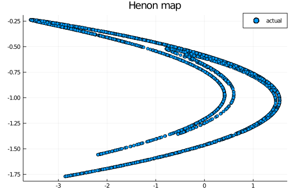
Now we want to venture into something that is not done in the paper: we want to see if this deterministic implementation of reservoirs and input layers are capable of reconstructing the Henon attractor. We will use the ESNs already built and we will predict the system for predict_len steps to see if the behaviour is manteined. We will do so only through an eye test, but it should suffice to have a general idea of the capabilities of these reservoirs.

To start we will plot the actual data, in order to have something to compare the resuls to:

scatter(test[1,:], test[2,:], label="actual")

actual

Now let’s see if the standard ESN is able to predict correctly this attractor

wout = ESNtrain(esn, beta)
output = ESNpredict(esn, predict_len, wout)
scatter(output[1,:], output[2,:], label="ESN")

ESN

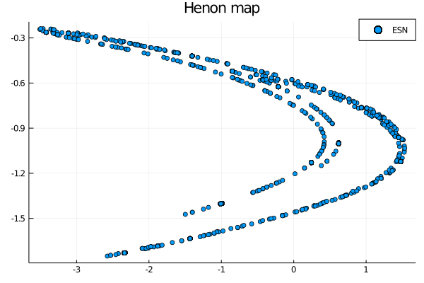
Not bad, but we already know the capabilities of the ESN. We are here to test the minimum complexity construction, so let us start with DLR

wout = ESNtrain(esndlr, beta)
output = ESNpredict(esndlr, predict_len, wout)
scatter(output[1,:], output[2,:], label="ESN-DLR")

ESN-DLR

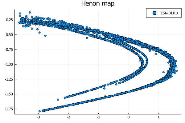
The predictions are not as clear cut as we would like, but the behaviour is manteined nevertheless. Actually impressive considering the simple construction of the reservoir. Trying the two other constructions gives the following:

wout = ESNtrain(esndlrb, beta)
output = ESNpredict(esndlrb, predict_len, wout)
scatter(output[1,:], output[2,:], label="ESN-DLRB")

ESN-DLRB

wout = ESNtrain(esnscr, beta)
output = ESNpredict(esnscr, predict_len, wout)
scatter(output[1,:], output[2,:], label="ESN-SCR")

ESN-SCR

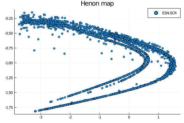
The results are somewhat similar between each other, and a deeper quantitative analysis is needed to determine the best performing construction, but this was not the aim of this post. We wanted to see if these basic implementations of reservoirs and input layers were capable not only of maintaining a short term prediction capability, but also if they were still able to mimic the behaviour of a chaotic attractor in the long term and it seems that both of these statements are proven to be correct. This seminal paper not only sheds light on the still inexplored possibilities of ESN reservoir constructions, but also shows that very little complexity is needed for this model to obtain very good results in a short amount of time.

As always, if you have any questions regarding the model, the package or you have found errors in my post, please don’t hesitate to contact me!

Citing

Part of the work done for this project has been published. If this post or the ReservoirComputing.jl software has been helpful, please consider citing the accompanying paper:

@article{JMLR:v23:22-0611,
  author  = {Francesco Martinuzzi and Chris Rackauckas and Anas Abdelrehim and Miguel D. Mahecha and Karin Mora},
  title   = {ReservoirComputing.jl: An Efficient and Modular Library for Reservoir Computing Models},
  journal = {Journal of Machine Learning Research},
  year    = {2022},
  volume  = {23},
  number  = {288},
  pages   = {1--8},
  url     = {http://jmlr.org/papers/v23/22-0611.html}
}

Documentation

[1] Rodan, Ali, and Peter Tino. “Minimum complexity echo state network.” IEEE transactions on neural networks 22.1 (2010): 131-144.

[2] Yildiz, Izzet B., Herbert Jaeger, and Stefan J. Kiebel. “Re-visiting the echo state property.” Neural networks 35 (2012): 1-9.

Minimum complexity reservoir and input layer#

Implementation in ReservoirComputing#

Example#

One step ahead prediction#

Attractor reconstruction#

Citing#

Documentation#