In the past few years a new framework based on the concept of Reservoir Computing has been proposed: the Cellular Automata based Reservoir Computer (ReCA) [1]. The advantage it proposes over standard implementations is given by the binary state of the reservoir and the fact that it doesn’t require much parameter tuning to obtain state of the art results. Since the initial conception of the use of ECA for reservoir computing numerous improvement have taken place. A recurrent design, together with the ReCA denomination, has been proposed in [2], and new methods for states encoding are studied in [3]. Also the use of two reservoir is studied in [4], as well as the implementation of two different rules, staked both horizontally [5] and vertically [6]. Lastly an exploration of complex rules is done in [7]. In this post we will illustrate the implementation in ReservoirComputing.jl of the general model, based on the architecture illustrated in [4] which build over the original implementation, improving the results. As always we will give an initial theoretical introduction, and then some examples of applications will be shown.
Reservoir Computing with Elementary Cellular Automata
Elementary Cellular Automata
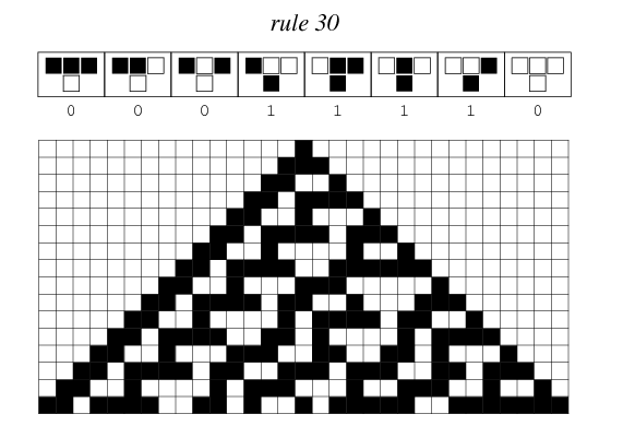
Initially introduced by Van Neumann as self-reproducing machines [8] Cellular Automata (CA) is a dynamical computational model based on a regular grid, of arbitrary dimensions, composed by cells. These cells can be in a different number of states and are updated according to a specific rule \( f \) which takes as an input the cell itself and its neighborhood and gives as output the state of the cell in the next generation. All the cells are updated simultaneously making the CA a discrete system with respect to time. The rule space is determined by the number of states and the number of possible neighbors. Let \( K \) be the number of states and \( S \) the the number of neighbors including the cell itself, then the possible number of neighborhood sates is given by \( K^S \). Since each element is transitioning to one of \( K \) states itself the transition function space is \( K^{K^S} \) [9]. Elementary cellular automata (ECA) are defined by a one dimensional grid of cells that are in one of two states, usually represented by 0 and 1. Each cell \( x \) updates its state \( x_i^t \) depending on the states of its two neighbors \( x_{i-1}^t \) and \( x_{i+1}^t \) according to the transition function \( f:{0,1}^3 \rightarrow {0,1} \). There are \( 2^8=256 \) elementary rules [10] that can be identified by numbers ranging from 0 to 255 taking the output table of each function as binary encoding of a digital number [11]. An example of rule 30 can be observed below.
Thanks to symmetries this rules con be grouped into 88 classes with equivalent characteristics [12]. Another distinction can be made, grouping the ECAs according to the general behavior they display. The first step in this direction was done by Wolfram [13], that identified four classes with the following description:
- Class 1: CA states evolve to a homogeneous behavior
- Class 2: CA states evolve periodically
- Class 3: CA states evolve with no defined pattern
- Class 4: can show all evolution patterns in an unpredictable manner
A more refined analysis by Li and Packard divided the Class 2 into two different sub-classes, distinguishing between fixed point and periodic CA. Class 3 rules are defined as globally chaotic and class 4 are considered difficult to include in specific categories.
ReCA Architecture
In the first stage the input needs to be mapped into the CA system. In the literature the ReCA approach has only been tested with binary test sets, so the chosen procedure for the input data is to translate directly the input onto the first state of the CA. In the original design [1] this was done by a random permutation of the elements of the input vector in a vector of the same dimension, $\text{L}_{\text{in}}$. The reservoir was then composed of \( \text{R} \) different ECA systems, each of which had a different random mapping as encoder. The evolution was done using the combination of the \( \text{R} \) reservoirs, so that the information could flow between one and the other. This approach yielded better results than letting them evolve separately. The starting vector for the ECA system is then the combination of the \( \text{R} \) mappings of the starting input vector, making it of dimensions $\text{R} \cdot \text{L}_{\text{in}}$.
An improvement over the here discussed method, proposed in [4], is to map the input into a different sized vector $\text{L}_{\text{d}}$, with $\text{L}_{\text{d}} > \text{L}_{\text{in}}$, padded with zeros. The higher dimension of the input vector allows the CA system to evolve with more freedom. Using a number of recombinations \( \text{R} \) the input vector to the CA system will be of dimensions $\text{R} \cdot \text{L}_{\text{d}}$. At the boundaries of the CA are used periodic boundary conditions (PBC), so that the last cell is neighbor with the first one.
Let $\text{X}_1$ be the first input vector. This will be randomly mapped onto a vector of zeros \( \text{R} \) times using a fixed mapping scheme $[\text{P}_1, \text{P}_2, …, \text{P}_{\text{R}}]$ and concatenated to form the initial configuration $\text{A}_0$ for the CA:
$$\text{A}_0^{(1)} = [\text{X}_{1}^{\text{P}_{1}}, \text{X}_{1}^{\text{P}_{2}}, …, \text{X}_{1}^{\text{P}_{\text{R}}}]$$
The transition function Z is then applied for I generations:
$$\text{A}_{1}^{(1)} = \text{Z}(\text{A}_0^{(1)})$$
$$\text{A}_{2}^{(1)} = \text{Z}(\text{A}_{1}^{(1)})$$
$$\vdots$$
$$\text{A}_{\text{I}}^{(1)} = \text{Z}(\text{A}_{\text{I}-1}^{(1)})$$
This constitutes the evolution of the CA given the input $\text{X}_1$. In the standard ReCA approach the state vector is the concatenation of all the steps $\text{A}_{1}^{(1)}$ through $\text{A}_{\text{I}}^{(1)}$ to form $\text{A}^{(1)} = [\text{A}_{1}^{(1)}, \text{A}_{2}^{(1)}, …, \text{A}_{\text{I}}^{(1)}]$.
The final states matrix, of dimensions $\text{R} \cdot \text{L}_{\text{d}} \times \text{T}$, is obtained stacking the state vectors column wise, in order to obtain: $\textbf{X}=[\text{A}^{(1) \text{T}}, \text{A}^{(2) \text{T}}, …, \text{A}^{(\text{T}) \text{T}}]$.
For the training technically every method we have implemented could be used, but in this first trial we just used the Ridge Regression. In the original paper the use of the pseudo-inverse was opted.
Implementation in ReservoirComputing.jl
Following the procedure described above we implemented in ReservoirComputing.jl a RECA_discrete object and a RECAdirect_predict_discrete function. The goal was to reproduce the results found in the literature, so the discrete approach was the only way to ensure that our implementation is correct. One of the goals is to expand this architecture to be also able to predict continuous values, such as timeseries. In this week an effort in this direction was made, but further exploration is needed. The RECA_discrete constructor takes as input
train_datathe data needed for the ReCA trainingrulethe ECA rule for the reservoirgenerationsthe number of generations the ECA will expand inexpansion_sizethe \( L_d \) parameterpermutationsthe number of additional ECA for the reservoir trainingnla_typethe non linear algorithm for the reservoir states. Default isNLADefalut()
The training is done using the already implemented ESNtrain, that will probably need a name change in the future since now it can train another family of Reservoir Computing models. The RECAdirect_predict_discrete function takes as input
recaan already constructedRECA_discreteW_outthe output ofESNtraintest_datathe input data for the direct prediction
Additionally a ECA constructor is also added to the package, taking as input the chosen rule, a vector of starting values starting_val and the number of generations for the ECA.
Examples
For testing the ReCA implementation we chose to solve the 5 bit memory task, a problem introduced in [14], a test proved to be hard for both Recurrent Neural Networks (RNN) and Echo State Networks (ESN), and fairly diffused in the ReCA literature.
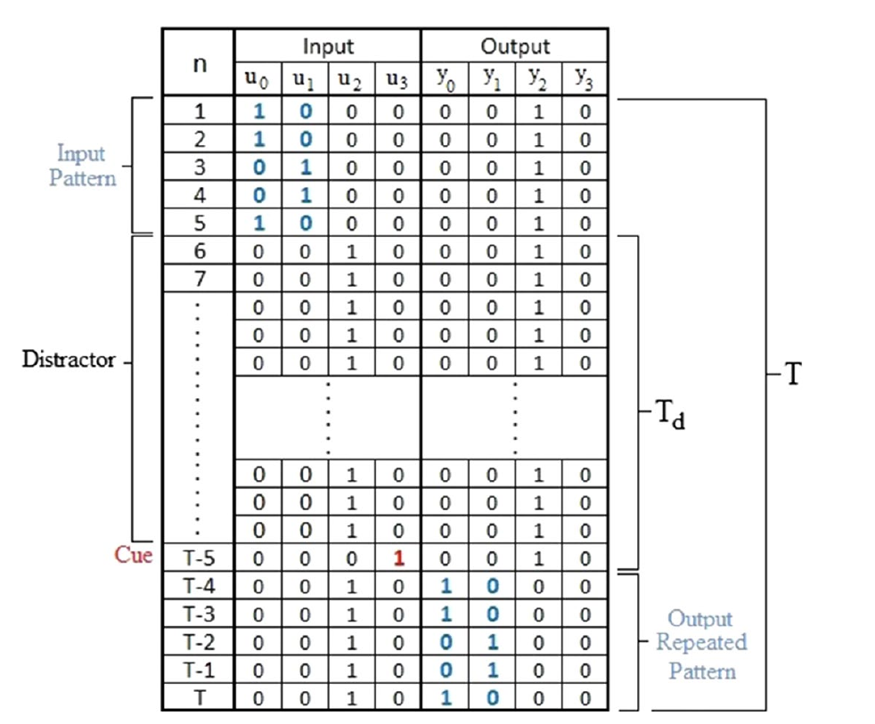
The test consists of four binary inputs and four binary outputs. In the first five timesteps of one run of the input sequence the first channel is one of the 32 possible five digit binary numbers, and the second input is complementary to the values in the first input (0, when the first channel is 1 and viceversa). The other two channels are zeros. This is the message that the model will have to remember. This is follow by a distractor period of $\text{T}_0$ steps, in which all the channels are zero with the exception of the third one, which is one up until $\text{T}_0-1$, where the fourth channel will be one and the third zero. This represents the cue. After that all channels except the third are zero.
For the output signal, all the channel are zero, but the third one which is one for all the steps with the exception of the last five, where the message from the input is repeated. A task is successful when the system is capable of reproducing all the $32 \times (5+\text{T}_0) \times 4$ bits of the output.
Below we can see an illustration [3] of the data contained in the 5 bit memory task:
Using a distractor period of \( \text{T}_0 = 200 \) and a value of \( \text{L}_d = 40 \) we tried to reproduce the results in the literature. In the table below are shown the successful run out of 100 performed, and the values in square indicates the number of generations and permutations, and are chosen in accordance to the values presented in the papers analized.
The lines of code needed for the training and prediction of the 5 bit memory task with the ReCA are the following:
reca = RECA_discrete(input, 60, 8, 40, 8)
W_out = ESNtrain(reca, 0.01, train_data = convert(AbstractArray{Float64}, output))
result = RECAdirect_predict_discrete(reca, W_out, input)
Where input and output are the datasets explained above, and the parameters to change for the results are rule, generations and permutations, in this example set to 60, 8, 8. Doing a cylce over each of them, for 100 runs we obtain the results below:
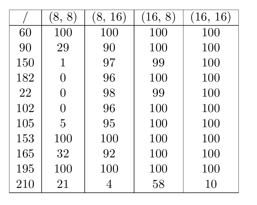
The values are in line with the results found in the literature, with little differences that could be attributed mainly to the training method. As already noted in the original paper, the computational power increases with the increasing of values of generations and permutations. It seems though that more generations is preferable over more permutations, since the (8, 16) correct runs are consistently less than the (16, 8) ones.
This model is really interesting, since it shows the capabilities of the Reservoir Computing approach. This family of models is still in its infancy, and a method for prediction of a continuous dataset is still missing. We hope that the implementation given in this package could help move the research in this direction.
As always, if you have any questions regarding the model, the package or you have found errors in my post, please don’t hesitate to contact me!
Citing
Part of the work done for this project has been published. If this post or the ReservoirComputing.jl software has been helpful, please consider citing the accompanying paper:
@article{JMLR:v23:22-0611,
  author  = {Francesco Martinuzzi and Chris Rackauckas and Anas Abdelrehim and Miguel D. Mahecha and Karin Mora},
  title   = {ReservoirComputing.jl: An Efficient and Modular Library for Reservoir Computing Models},
  journal = {Journal of Machine Learning Research},
  year    = {2022},
  volume  = {23},
  number  = {288},
  pages   = {1--8},
  url     = {http://jmlr.org/papers/v23/22-0611.html}
}
Documentation
[1] Yilmaz, Ozgur. “Reservoir computing using cellular automata.” arXiv preprint arXiv:1410.0162 (2014).
[2] Margem, Mrwan, and Ozgür Yilmaz. “An experimental study on cellular automata reservoir in pathological sequence learning tasks.” (2017).
[3] Margem, Mrwan, and Osman S. Gedik. “Feed-forward versus recurrent architecture and local versus cellular automata distributed representation in reservoir computing for sequence memory learning.” Artificial Intelligence Review (2020): 1-30.
[4] Nichele, Stefano, and Andreas Molund. “Deep reservoir computing using cellular automata.” arXiv preprint arXiv:1703.02806 (2017).
[5] Nichele, Stefano, and Magnus S. Gundersen. “Reservoir computing using non-uniform binary cellular automata.” arXiv preprint arXiv:1702.03812 (2017).
[6] McDonald, Nathan. “Reservoir computing & extreme learning machines using pairs of cellular automata rules.” 2017 International Joint Conference on Neural Networks (IJCNN). IEEE, 2017.
[7] Babson, Neil, and Christof Teuscher. “Reservoir Computing with Complex Cellular Automata.” Complex Systems 28.4 (2019).
[8] Neumann, János, and Arthur W. Burks. Theory of self-reproducing automata. Vol. 1102024. Urbana: University of Illinois press, 1966.
[9] Bia_ynicki-Birula, Iwo, and Iwo Bialynicki-Birula. Modeling Reality: How computers mirror life. Vol. 1. Oxford University Press on Demand, 2004.
[10] Wolfram, Stephen. A new kind of science. Vol. 5. Champaign, IL: Wolfram media, 2002.
[11] Adamatzky, Andrew, and Genaro J. Martinez. “On generative morphological diversity of elementary cellular automata.” Kybernetes (2010).
[12] Wuensche, Andrew, Mike Lesser, and Michael J. Lesser. Global Dynamics of Cellular Automata: An Atlas of Basin of Attraction Fields of One-Dimensional Cellular Automata. Vol. 1. Andrew Wuensche, 1992.
[13] Wolfram, Stephen. “Universality and complexity in cellular automata.” Physica D: Nonlinear Phenomena 10.1-2 (1984): 1-35.
[14] Hochreiter, Sepp, and Jürgen Schmidhuber. “Long short-term memory.” Neural computation 9.8 (1997): 1735-1780.