Continuing the work started last week we are going to further explore the capabilities of Reservoir Computing using Cellular Automata (CA) as the reservoir. As always a little theorical introduction is given and then we will illustrate the use of the model implemented in ReservoirComputing.jl.

Reservoir Computing with Two Dimensional Cellular Automata

Two Dimensional Cellular Automata (Conway’s Game of Life)

In the previous week we used Elementary CA (ECA) to train our model, and this time we want to see if we are able to obtain similar results using a two dimensional CA. As proposed in [1] we are going to use Conway’s Game of Life [2] (GoL), so a little introduction to this model is essential to proceed.

Conway’s Game of Life (GoL) is an example of two-dimensional CA with a Moore neighborhood with range $r=1$ [3], defined as:

$$ N^{M}_{(x_0, y_0)} = {(x, y):|x-x_0| \le r, |y-y_0| \le r } $$

where $(x_0, y_0)$ is the given cell. In the standard GoL format each cell in the grid can be in either of two states: dead or alive (identified respectively with 0 and 1). The transition rules are determined as follows:

Any alive cell with fewer than two alive cells in its neighborhood will transition to a dead state in the next generation
Any alive cell with two or three alive cells in its neighborhood will remain alive in the next generation
Any alive cell with more than three alive neighbors will transition to a dead state in the next generation
Any dead cell with three alive neighbors will transition to an alive state in the next generation

This CA shows class 4 behavior, neither completely random nor completely repetitive. It is also capable of universal computation and it’s Turing complete [4].

We can obtain a GIF of the system using the package ReservoirComputing and Plots in a couple of lines of code: first let’s import the packages

using ReservoirComputing
using Plots

We can now define the variables for the GoL CA, namely dimensions and generations, and defining the GoL object at the same time:

size = 100
generations = 250
@time gol = GameOfLife(rand(Bool, size, size), generations);

0.091884 seconds (8 allocations: 2.394 MiB)

and now we can plot the obtiained GoL system:

@gif for i=1:generations
    heatmap(gol.all_runs[:, :, i], color=cgrad([:white,:black]),
    legend = :none,
    axis=false)
    plot!(size=(500,500))
end

tmp

As we can see, starting from a random position, we obtained an evolving GoL system.

Game of Life reservoir Architecture

Since the data used for testing in the literature is also binary in nature, in order to feed it to the reservoir, the method proposed in [1] was based on randomly projecting the input data into the reservoir, whose size should follow that of the input data. This means that for an input of dimension $L_{in}=4$ the size of the reservoir would have been $m=2 \times 2$. This procedure was repeated a number $R$ of times, effectively creating $R$ different reservoirs. These reservoirs were then connected and the information was allowed to flow between them, in order to obtain an higher dimensional reservoir. This architecture has showed the capability to correctly solve the 5 bit and 20 bit memory task.

In the implementation in ReservoirComputing.jl we want to propose an expansion of the encoding method, also capable of solving the 5 bit memory task. Following intuitions given by more recent papers in the field of ReCA, in particular [5] and [6], we decided to input the data to the reservoir using $T$ random projections into an higher dimension matrix. This way the initial state has room to expand and memory of the precedent state is conserved. The procedure is similar to that described by [1], and is illustrated in the figure.

encoding

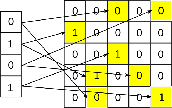
Let $\text{X}_1$ be the first input vector. This will be randomly mapped onto a matrix of zeros $T$ times using a fixed mapping scheme $[\text{P}_1, \text{P}_2, …, \text{P}_{\text{R}}]$ in order to form the initial configuration $\text{A}_0^{(1)}$ for the GoL. The transition function $Z$, the rules of GoL, is then applied for $I$ generations:

$$\text{A}_{1}^{(1)}=\text{Z}(\text{A}_0^{(1)})$$

$$ \text{A}_{2}^{(1)} = \text{Z}(\text{A}_{1}^{(1)}) $$

$$ \vdots $$

$$ \text{A}_{\text{I}}^{(1)} = \text{Z}(\text{A}_{\text{I}-1}^{(1)}) $$

This constitutes the evolution of the CA given the input $\text{X}_1$. In order to create the state vector we need to vectorize and concatenate the matrices we obtained. Identifying with $\text{A}_{0, 1}^{(1)}$ the first column of $\text{A}_0^{(1)}$, let $c$ be the total number of columns of $\text{A}_0^{(1)}$, then the vectorization of $\text{A}_0^{(1)}$ will be

$$\text{v}\text{A}_0^{(1)} = [\text{A}_{0, 1}^{(1)}, \text{A}_{0, 2}^{(1)}, …, \text{A}_{0, c}^{(1)}]$$

This procedure is done for every timestep $I$, and at the end the vector state $\textbf{x}^{(1)}$ will be

$$\textbf{x}^{(1)} = [\text{v}\text{A}_0^{(1)}, \text{v}\text{A}_1^{(1)}, …, \text{v}\text{A}_{I}^{(1)}]$$

An illustration of this process can be seen in figure.

stateharvest

To feed the second input vector $\text{X}_2$ we use the same mapping created in the first step. Instead of using an initial empty matrix this time we will project the input over the matrix representing the last evolution of the prior step, $\text{A}_{\text{I}}^{(1)}$. The matrix thus obtained is evolved as described above, to obtain the state vectors for the second input vector. This procedure is repeated for every input vector.

The training is carried out using Ridge Regression.

Example

For example we will try to reproduce the 5 bit memory task, described last week. If you want to follow along and experiment with the model, the data can be found here: the 5bitinput.txt is the input data and the 5bitoutput is the desired output. To read the data we can use the following

using DelimitedFiles

input = readdlm("./5bitinput.txt", ',', Int)
output = readdlm("./5bitoutput.txt", ',', Int)

Now that we have the data we can train the model and see if it is capable of solving the 5 bit memory task with a distractor period of 200.

using ReservoirComputing

reca = RECA_TwoDim(input, 30, 10, 110)
W_out = ESNtrain(reca, 0.001; train_data = convert(AbstractArray{Float64}, output))
reca_output = RECATDdirect_predict_discrete(reca, W_out, input)
reca_output == output

true

It seems that for architecture used in this example the task is easily solvable. A more deep investigation can be made iterating over different values of reservoir size, permutations and generations, but it can take some time. The results for 100 runs for some of the combinations are given in the table below:

table2

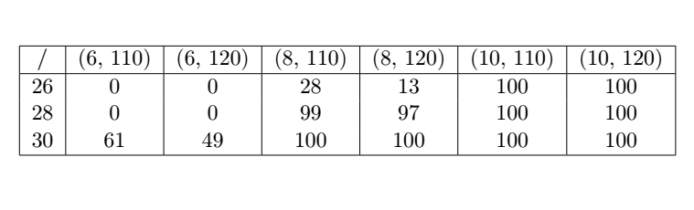
where (n, m) stands for n = generations and m = permutations. The sizes chosen for the system are 26, 28 and 30. As we can see for some of these parameters the 5 bit memory task is solved 100 times out of 100 runs.

As always, if you have any questions regarding the model, the package or you have found errors in my post, please don’t hesitate to contact me!

Citing

Part of the work done for this project has been published. If this post or the ReservoirComputing.jl software has been helpful, please consider citing the accompanying paper:

@article{JMLR:v23:22-0611,
  author  = {Francesco Martinuzzi and Chris Rackauckas and Anas Abdelrehim and Miguel D. Mahecha and Karin Mora},
  title   = {ReservoirComputing.jl: An Efficient and Modular Library for Reservoir Computing Models},
  journal = {Journal of Machine Learning Research},
  year    = {2022},
  volume  = {23},
  number  = {288},
  pages   = {1--8},
  url     = {http://jmlr.org/papers/v23/22-0611.html}
}

Documentation

[1] Yilmaz, Ozgur. “Reservoir computing using cellular automata.” arXiv preprint arXiv:1410.0162 (2014).

[2] Gardner, Martin. “Mathematical games: The fantastic combinations of John Conway’s new solitaire game “life”.” Scientific American 223.4 (1970): 120-123.

[3] Weisstein, Eric W. “Moore Neighborhood.” From MathWorld–A Wolfram Web Resource. https://mathworld.wolfram.com/MooreNeighborhood.html

[4] Wolfram, Stephen. A new kind of science. Vol. 5. Champaign, IL: Wolfram media, 2002.

[5] Margem, Mrwan, and Osman S. Gedik. “Feed-forward versus recurrent architecture and local versus cellular automata distributed representation in reservoir computing for sequence memory learning.” Artificial Intelligence Review (2020): 1-30.

[6] Nichele, Stefano, and Andreas Molund. “Deep reservoir computing using cellular automata.” arXiv preprint arXiv:1703.02806 (2017).

Reservoir Computing with Two Dimensional Cellular Automata#

Two Dimensional Cellular Automata (Conway’s Game of Life)#

Game of Life reservoir Architecture#

Example#

Citing#

Documentation#