This week body of work is less then the usual amount, since most of my time was spent watching the incredible talks given at JuliaCon 2020. This was my first time attending and I just wanted to spend a few lines congratulating all the speakers for the amazing work they are doing with Julia, and most importantly I wanted to thank the organizers for the fantastic job they did: it really felt like an actual physical conference and the sense of community was truly awesome to experience.

In the middle of all the talks I was still able to read a couple of papers and write some code, and this week work is a companion to the work done in week 6: expanding the research done in their previous article [1], they constructed a different type of cycle reservoir with random jumps and a different way to create an input layer [2]. In this post we will discuss the theory expressed in the paper and, after explaining the implementation in ReservoirComputing.jl, we will show how this construction performs on the tasks we takled in week 6.

Cycle Reservoirs with Jumps and irrational sign input layer

The costruction of Cycle Reservoirs with Jumps (CRJ) builds over the idea of the Simple Cycle Reservoir (SCR): contrary to the stadard construction of an Echo State Network (ESN) standard reservoir the two algorithms proposed are completely deterministic and really simple in nature. In the CRJ model the reservoir nodes are connected in a unidirectional cycle, as they are in the SCR model, with bidirectional shortcuts (called jumps). The value for the cycle connections are the same $ r_c > 0 $, and all the jumps also share the same values $ r_j > 0 $. The construction of the CRJ reservoir can be described in the following way:

The lower subdiagonal of the reservoir $ \textbf{W} $ is equal to the chosen $ r_c $
The upper right corner of reservoir $ \textbf{W} $ is equal to the chosen $ r_c $
With a chosen jump size $ 1 < l < [N/2] $ if $ (N \text{mod}l) = 0 $ then there are $ [N/l] $ jumps, the first being from unit 1 to unit $ 1+l $, the last from unit $ N+1-l $ to unit 1. If $ (N \text{mod}l) \ne 0 $ then there are $ [N/l] $ jumps, the last jump ending in unit $ N+1-(N\text{mod}l) $. All the jumps have the same chosen value $ r_j $

Along with the construction of the CRJ model the paper [2] proposes a fully connected input layer with the same absolute value of the connection weight. The sign of the input weights is determined using the decimal expansion of an irrational number, $ \pi $ being the choice of the authors. The first $ N $ digits $ d_1, d_2,…,d_N $ are taken and if $ 0 \le d_n \le 4 $ then the nth input will have sign - (minus), else if $ 5 \le d_n \le 9 $ it will have a + (plus) sign.

Implementation in ReservoirComputing

A new function called CRJ() has been added to the reservoirs construction; this function takes as input

res_size the size of the reservior
cyrcle_weight the value of the weights $ r_c $
jump_weight the value of the weights $ r_j $
jump_size the number of jumps $ l $

and gives as output a reservoir matrix. In addition a function for the construction of the input layer has also been added. Denominated irrational_sign_input() it takes as input

res_size the size of the reservior
in_size the size of the input vector
weight the absolute value of the connection weight
irrational an optionl input, with default $ \pi $, used for the determination of the sign for the connection weights

Example

To remain in line with the work done in the 6th week, and in order to be able to do a meaningful comparison, we are going to use the Henon map for our tests. The Henon map is defined as

$$x_{x+1} = 1 - ax_n^2 + y_n$$ $$ y_{n+1} = bx_n $$

To obtaine the data for out tests we are going to use DynamicalSystems.jl. Before starting the work let’s download and inport all useful packages

using Pkg
Pkg.add("ReservoirComputing")
Pkg.add("Plots")
Pkg.add("DynamicalSystems")
Pkg.add("LinearAlgebra")
Pkg.add("Random")

using ReservoirComputing
using Plots
using DynamicalSystems
using LinearAlgebra
using Random

Now we can generate the Henon map, and we will shift the data points by -0.5 and scale them by 2 to reproduce the data we had last time. The initial transient will be washed out and we will create two datasets called train and test:

ds = Systems.henon()
traj = trajectory(ds, 7000)
data = Matrix(traj)'

data = (data .-0.5) .* 2
shift = 200
train_len = 2000
predict_len = 3000
train = data[:, shift:shift+train_len-1]
test = data[:, shift+train_len:shift+train_len+predict_len-1]

Having the needed data we can proceed to the prediction tasks.

One step ahead prediction

For sake of comparison we are going to use the same values as last time for the construction of the ESN:

approx_res_size = 100
radius = 0.3
sparsity = 0.5
sigma = 1.0
beta = 1*10^(-1)
extended_states = true

input_weight = 0.95
cyrcle_weight = 0.95
jump_weight = 0.2
jumps = 5

Since this task was not used in the paper [2] the new parameters jump_weight and jumps are obtained using a manual grid search and as such are probably not as optimized as the other values. We can proceed to the construction of the ESN with the CRJ reservoir and irrational-determined input layer:

@time W = CRJ(approx_res_size, cyrcle_weight, jump_weight, jumps)
W_in = irrational_sign_input(approx_res_size, size(train, 1), input_weight)
esn_crj = ESN(W, train, W_in, extended_states = extended_states)

0.000053 seconds (6 allocations: 78.359 KiB)

Following the procedure we used lst time, in order to test the accuracy of the prediction we are going to use the Normalized Mean Square Error (NMSE), defined as

$$NMSE = \frac{<||\hat{y}(t)-y(t)||^2>}{<||y(t)-<y(t)>||^2>}$$

where

$ \hat{y}(t) $ is the readout output
$ y(t) $ is the target output
$ <\cdot> $ indicates the empirical mean
$ ||\cdot|| $ is the Euclidean norm.

A simple NMSE function can be created following:

function NMSE(target, output)
    num = 0.0
    den = 0.0
    sums = []
    for i=1:size(target, 1)
        append!(sums, sum(target[i,:]))
    end
    for i=1:size(target, 2)
        num += norm(output[:,i]-target[:,i])^2.0
        den += norm(target[:,i]-sums./size(target, 2))^2.0
    end
    nmse = (num/size(target, 2))/(den/size(target, 2))
    return nmse
end

Testing the one step ahead predicting capabilities of this new implementation we obtain:

wout = ESNtrain(esn_crj, beta)
output = ESNpredict_h_steps(esn_crj, predict_len, 1, test, wout)
println(NMSE(test, output))

0.0010032069150514866

This result outperforms all the architectures tested in week 6, getting a little closer to the standard ESN implementation result. Even though this task is not present in the paper the better results shows that the implementation is valid nevertheless.

Attractor reconstruction

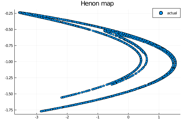
Following the work done in week 6 we want to explore the capabilities of this construction in the reconstruction of the chaotic attractor of the Henon map. Using the already built ESN we will predict the system for predict_len steps and at the end we will plot the results to see if they are in line with the one obtained with the other architectures. To refresh our memory we will start by plotting the actual Henon map:

scatter(test[1,:], test[2,:], label="actual")

actual

Let’s see if the CRJ-based ESN is capable of reproducing the climate of this attractor:

wout = ESNtrain(esn_crj, beta)
output = ESNpredict(esn_crj, predict_len, wout)
scatter(output[1,:], output[2, :], lable = "ESN-CRJ")

ESN-CRJ

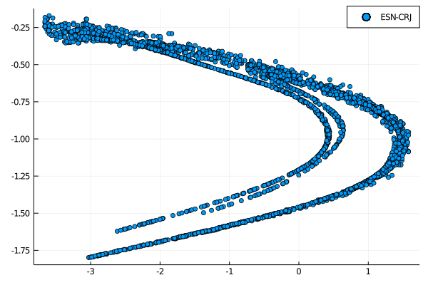
The result is actually more clear cut then the results obtained in the 6th week. This architecture seems to be able to represent the attractor in a more precise manner. Both the tests we have done have resulted in a better performance with respect to the other deterministic constructions for reservoirs and input layer. A more statistical accurate exploration is of course needed but both our results and the results found in the paper show the capabilities of this new implementation of a deterministic reservoir.

As always, if you have any questions regarding the model, the package or you have found errors in my post, please don’t hesitate to contact me!

Citing

Part of the work done for this project has been published. If this post or the ReservoirComputing.jl software has been helpful, please consider citing the accompanying paper:

@article{JMLR:v23:22-0611,
  author  = {Francesco Martinuzzi and Chris Rackauckas and Anas Abdelrehim and Miguel D. Mahecha and Karin Mora},
  title   = {ReservoirComputing.jl: An Efficient and Modular Library for Reservoir Computing Models},
  journal = {Journal of Machine Learning Research},
  year    = {2022},
  volume  = {23},
  number  = {288},
  pages   = {1--8},
  url     = {http://jmlr.org/papers/v23/22-0611.html}
}

Documentation

[1] Rodan, Ali, and Peter Tino. “Minimum complexity echo state network.” IEEE transactions on neural networks 22.1 (2010): 131-144.

[2] Rodan, Ali, and Peter Tiňo. “Simple deterministically constructed cycle reservoirs with regular jumps.” Neural computation 24.7 (2012): 1822-1852.

Cycle Reservoirs with Jumps and irrational sign input layer#

Implementation in ReservoirComputing#

Example#

One step ahead prediction#

Attractor reconstruction#

Citing#

Documentation#