Following an architecture found on [1] this week we decided to implement a reservoir model based on the Gated Recurring Unit (GRU) structure, first described in [2]. This architecture is an evolution of the standard Recurrent Neural Network (RNN) update equations and works in a similar way to Long Short Term Memory (LSTM) with a forget gate but with fewer parameters; the LSTM usually outperfofms the GRU in most task but it could be interesting to see the behavior of this unit in the Echo State Network (ESN) model. In the first part of this post we will briefly explain the theory behind the model and after we will show an example to see the performance of this architecture.

Gated Recurring Unit

As described in [2] the update equations in the GRU hidden unit are described as follows:

The reset gate is computed by $$\textbf{r}_t = \sigma (\textbf{W}_r \textbf{x}_t + \textbf{U}_r \textbf{h}_{t-1} + \textbf{b}_r)$$ where $ \sigma $ is the sigmoid function. $ \textbf{x}_t $ is the input at time $ t $ and $ \textbf{h}_{t-1} $ is the previous hidden state. In the ESN case it will be the provious state vector.
In a similar way, the update gate is computed by $$\textbf{z}_t = \sigma (\textbf{W}_z \textbf{x}_t + \textbf{U}_z \textbf{h}_{t-1} + \textbf{b}_z)$$
The candidate activation vector is given by $$\tilde{\textbf{h}}_t = f(\textbf{W}_h \textbf{x}_t + \textbf{U}_h (\textbf{r}_t \circ \textbf{h}_{t-1}) + \textbf{b}_h)$$ where $ \circ $ represents the Hadamard product. In the ESN case $ \textbf{U}_h = \textbf{W}, \textbf{W}_h = \textbf{W}_in $ where $ \textbf{W} $ is the reservoir matrix and $ \textbf{W}_in $ is the input layer matrix. In the original implementation the activation function $ f $ is taken to be the hyperbolic tangent.
The final states vector is given by $$\textbf{h}_t = (1-\textbf{z}_t) \circ \textbf{h}_{t-1} + \textbf{z}_t \circ \tilde{\textbf{h}}_t$$

Alternative forms are known but for the first implementation we decided to focus more our attention on the standard model. The $ \textbf{W}, \textbf{U} $ layers are fixed and constructed using the irrational number input layer generator (see [3] or week 9), with a different start for the change of sign but in the future we would like to give more possibilities for the construction of these layers.

Implementation in ReservoirComputing

The overall implementation is not the hardest part, band following the instructions of the original paper we were able to implement a gru base function that updates the states vector at every time step. Building on that function we implemented two public function, the constructor GRUESN and the predictor GRUESNpredict. The first one takes as input the same inputs as the ESN constructor with the addition of the gates_weight optional value, set to 0.9 as default. The GRUESNpredict function takes as input the same values as the ESNpredict function and return the prediction made by the GRUESN.

Example

Since this model isn not found in literature, only as comparison in [1] but for different tasks than time series prediction, we chose to use yet again the Henon map to test the capabilities of this model in the reproduction of a choatic system. This particular model was chosen since is less complex than the Lorenz system and it requires little parameter tuning in order to obtain decent results.

Let us start by insalling and importing the usual packages

using Pkg
Pkg.add("ReservoirComputing")
Pkg.add("DynamicalSystems")
Pkg.add("Plots")

using ReservoirComputing
using DynamicalSystems
using Plots

The construction of the Henon map is straight forward. Again the data points are shifted by -0.5 and scaled by 2:

ds = Systems.henon()
traj = trajectory(ds, 7000)
data = Matrix(traj)'

data = (data .-0.5) .* 2
shift = 200
train_len = 2000
predict_len = 3000
train = data[:, shift:shift+train_len-1]
test = data[:, shift+train_len:shift+train_len+predict_len-1]

For this example we will use the irrational sign input matrix in order to be consistent with the construction of the GRU unit, and for the reservoir matrix we will use the standard implementation

approx_res_size = 100
radius = 0.99
sparsity = 0.1
sigma = 1.0
beta = 1*10^(-1)
extended_states = false
input_weight = 0.1

W = init_reservoir_givensp(approx_res_size, radius, sparsity)
W_in = irrational_sign_input(approx_res_size, size(train, 1), input_weight)
@time gruesn = GRUESN(W, train, W_in, extended_states = extended_states, gates_weight = 0.8)

0.286364 seconds (51.78 k allocations: 36.200 MiB, 13.94% gc time)

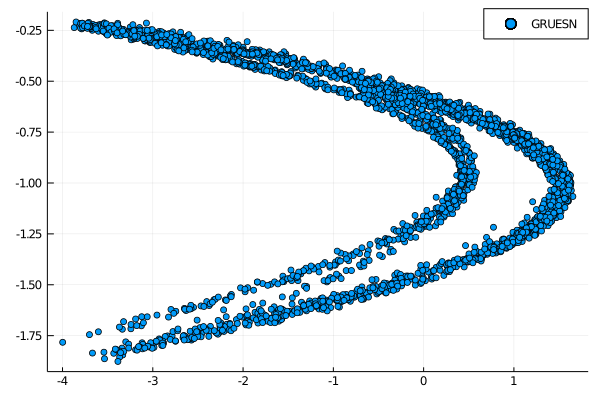
The parameters were chosen by manual grid search, so it is possibile that they are not the best ones for this task. A more in depth research will be needed for this specific prediction. Using these values we can train the GRUESN and make a prediction. We will scatter the results after in order to compare the prediction obtained

W_out = ESNtrain(gruesn, beta)
output = GRUESNpredict(gruesn, predict_len, W_out)
scatter(output[1,:], output[2, :], lable = "ESN-CRJ")

gruesn

The actual Henon map is the following

scatter(test[1,:], test[2,:], label="actual")

actual

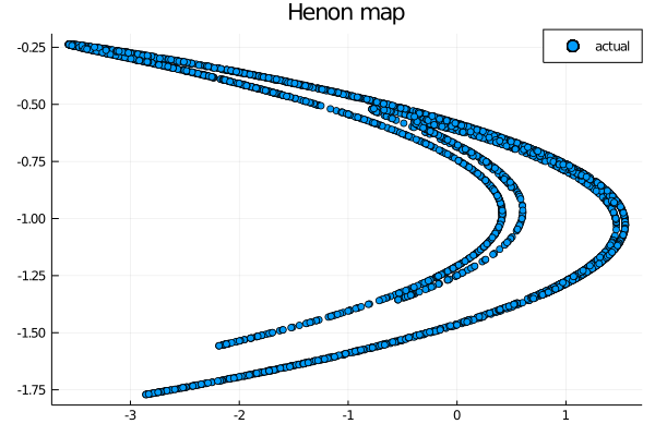
As we can see the model is able to replicate the behavior of the chaotic system up to a certain degree. The prediction is not as clear cut as others taht we were able to obtain but it shows the potential of this model, given more time for the parameters tuning. Using a different construction for the hidden layers could also help in improving the predictive capabilities.

As always, if you have any questions regarding the model, the package or you have found errors in my post, please don’t hesitate to contact me!

Citing

Part of the work done for this project has been published. If this post or the ReservoirComputing.jl software has been helpful, please consider citing the accompanying paper:

@article{JMLR:v23:22-0611,
  author  = {Francesco Martinuzzi and Chris Rackauckas and Anas Abdelrehim and Miguel D. Mahecha and Karin Mora},
  title   = {ReservoirComputing.jl: An Efficient and Modular Library for Reservoir Computing Models},
  journal = {Journal of Machine Learning Research},
  year    = {2022},
  volume  = {23},
  number  = {288},
  pages   = {1--8},
  url     = {http://jmlr.org/papers/v23/22-0611.html}
}

Documentation

[1] Paaßen, Benjamin, and Alexander Schulz. “Reservoir memory machines.” arXiv preprint arXiv:2003.04793 (2020).

[2] Cho, Kyunghyun, et al. “Learning phrase representations using RNN encoder-decoder for statistical machine translation.” arXiv preprint arXiv:1406.1078 (2014).

[2] Rodan, Ali, and Peter Tiňo. “Simple deterministically constructed cycle reservoirs with regular jumps.” Neural computation 24.7 (2012): 1822-1852.

Gated Recurring Unit#

Implementation in ReservoirComputing#

Example#

Citing#

Documentation#

Gated Recurring Unit

Implementation in ReservoirComputing

Example

Citing

Documentation