This post is meant to work as an high level introduction to the concept of Reservoir Computing, using the Julia package ReservoirComputing.jl as example tool. This package is a work in progress and it is currently the main project I am working on as part of the Google Summer of Code program. Future posts are going to further explain the various implementations and improvements to the code by means of comparisons with the literature and examples.

What is Reservoir Computing?

Reservoir Computing is an umbrella term used to identify a general framework of computation derived from Recurrent Neural Networks (RNN), indipendently developed by Jaeger [1] and Maass et al. [2]. These papers introduced the concepts of Echo State Networks (ESN) and Liquid State Machines (LSM) respectively. Further improvements over these two models constitute what is now called the field of Reservoir Computing. The main idea lies in leveraging a fixed non-linear system, of higher dimension than the input, onto which to input signal is mapped. After this mapping is only necessary to use a simple readout layer to harvest the state of the reservoir and to train it to the desired output. In principle, given a complex enough system, this architecture should be capable of any computation [3]. The intuition was born from the fact that in training RNNs most of the times the weights showing most change were the ones in the last layer [4]. In the next section we will also see that ESNs actually use a fixed random RNN as the reservoir. Given the static nature of this implementation usually ESNs can yield faster results and in some cases even better, in particular when dealing with chaotic time series predictions [5].

But not every complex system is suited to be a good reservoir. A good reservoir is one that is able to separate inputs; different external inputs should drive the system to different regions of the configuration space [3]. This is called the separability condition. Furthermore an important property for the reservoirs of ESNs is the Echo State property which states that inputs to the reservoir echo in the system forever, or util they dissipate. A more formal definition of this property can be found in [6].

In order to better show the inner workings of models of this family I am going to explain in mathematical details the ESN, a model that is already implemented in the package, so it will be useful for making examples.

Echo State Networks

Theoretical Background

This intends to be a quick overview of the theory behind the ESN to get the reader acquainted with the concepts and workings of this particular model, and it is by no means comprehensive. For in depth reviews and explanations please refer to [7] and [8]. All of the information laid out in this section is adapted from these two sources, unless stated otherwise.

Let us suppose we have an input signal \( \textbf{u}(t) \in R^M \) where \( t = 1, …, T \) is the discrete time and \( T \) the number of data points in the training set. In order to project this input onto the reservoir we will need an input to reservoir coupler, identified by the matrix \( \textbf{W}_{\text{in}} \in R^{N \times M} \). Usually this matrix is built in the same way the reservior is, and at the same time. For the implementation used in ReservoirComputing.jl we have followed the same construction proposed in [9] where the i-th of the \( M \) input signals is connected to \( N/M \) reservoir nodes with connection weights in the i-th column of \( \textbf{W}_{\text{in}} \). The non-zero elements are chosen randomly from a uniform distribution and then scaled in the range \( [-\sigma , \sigma ] \).

The reservoir is constitued by \( N \) neurons connected in a Erdős–Rényi graph configuration and it is represented by an adjacency matrix \( \textbf{W} \) of size \( N \times N \) with values drawn from a uniform random distribution on the interval \( [-1, 1] \) [5]. This is the most important aspect of the ESN, so in order to build one in an efficient manner we must first understand all of its components.

• The size \( N \) is of course the single most important one: the more challenging the task, the bigger the size should be. Of course a bigger matrix will mean more computational time so the advice of Lukoševičius is to start small and then scale.
• The sparsity of the reservoir. In most papers we see that each reservoir node is connected to a small number of other nodes, ranging from 5 to 12. The sparseness, beside theoretical implications, is also useful to speed up computations.
• Spectral radius. After the generation of a random sparse reservoir matrix, its spectral radius \( \rho (\textbf{W}) \) is computed and \( \textbf{W} \) is divided by it. This allows us to obtain a matrix with a unit spectral radius, that can be scaled to a more suited value. Altough there are exceptions (when the inputs \( \textbf{u}(t) \) are non-zero for example), a spectral radius smaller than unity \( \rho (\textbf{W}) < 1 \) ensures the echo state property. More generally this parameter should be selected to maximize the performance, keeping the unitary value as a useful reference point.

After the construction of the input layer and the reservoir we can focus on harvesting the states. The update equations of the ESN are:

$$\textbf{x}(t) = (1-\alpha) \textbf{x}(t-1)+\alpha f( \textbf{W} \textbf{x}(t-1)+ \textbf{W}_{\text{in}} \textbf{u}(t))$$

$$\textbf{v}(t) = g( \textbf{W}_{\text{out}} \textbf{x}(t))$$

where

• \( \textbf{v}(t) \in R^{M} \) is the predicted output
• \( \textbf{x}(t) \in R^{N} \) is the state vector
• \( \textbf{W}_{\text{out}} \in R^{M \times N} \) is the output layer
• \( f \) and \( g \) are two activation functions, most commonly the hyperbolic tangent and identity respectively
• \( \alpha \) is the leaking rate

The computation of \( \textbf{W}_{\text{out}} \) can be expressed in terms of solving a system of linear equations

$$\textbf{Y}^{\text{target}}=\textbf{W}_{\text{out}} \textbf{X}$$

where \( \textbf{X} \) is the states matrix, built using the single states vector \( \textbf{x}(t) \) as column for every \( t=1, …, T \), and \( \textbf{Y}^{\text{target}} \) is built in the same way only using \( \textbf{y}^{\text{target}}(t) \). The chosen solution for this problem is usually the Tikhonov regularization, also called ridge regression which has the following close form:

$$\textbf{W}_{\text{out}} = \textbf{Y}^{\text{target}} \textbf{X}^{\text{T}}(\textbf{X} \textbf{X}^{\text{T}} + \beta \textbf{I})^{-1}$$

where \( \textbf{I} \) is the identity matrix and \(\beta \) is a regularization coefficient.

After the training of the ESN, the prediction phase uses the same update equations showed above, but the input \( \textbf{u}(t) \) is represented by the computed output \( \textbf{v}(t-\Delta t) \) of the preceding step.

In short this is the core theory behind the ESNs. In order to visualize how they work let’s look at an example.

Lorenz system prediction

This is a task already tackled in literature, so our intent is to try and replicate the results found in [10]. This example can be followed in its entirety here. In this section we will just give part of the code to illustrate the theory explained above, so some important parts are not displayed.

Supposing we have already created the train data, constituted by 5000 timesteps of the chaotic Lorenz system, we are going to use the same parameters found in the paper:

using ReservoirComputing
approx_res_size = 300
radius = 1.2
degree = 6
activation = tanh
sigma = 0.1
beta = 0.0
alpha = 1.0
nla_type = NLAT2()
extended_states = false

The ESN can easily be called in the following way:

esn = ESN(approx_res_size,
    train,
    degree,
    radius,
    activation, #default = tanh
    alpha, #default = 1.0
    sigma, #default = 0.1
    nla_type #default = NLADefault(),
    extended_states #default = false
    )

The training and the prediction, for 1250 timestps, are carried out as follows

W_out = ESNtrain(esn, beta)
output = ESNpredict(esn, predict_len, W_out)

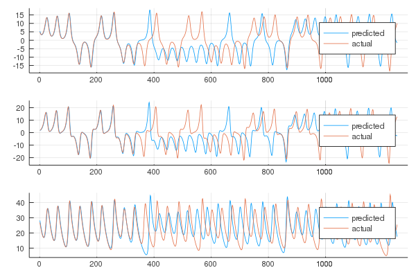
In order to visualize the solution we can plot the individual trajectories

and the attractors

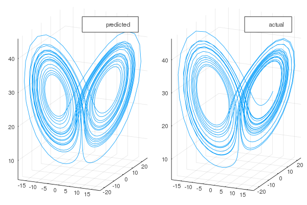
As expected the short term predictions are very good, and in the long term the behaviour of the system is mantained.

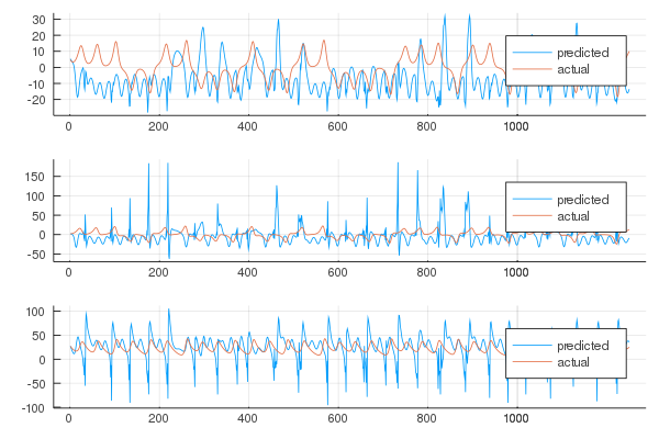
But what happens if the parameters are not ideal? In the paper is given an example where the spectral radius is bigger than the ideal value and the predictions are compromised as a result. We can also show that if the value is less than one, as suggested in order to mantain the echo state property, the results are nowhere near optimal.

radius = 0.8

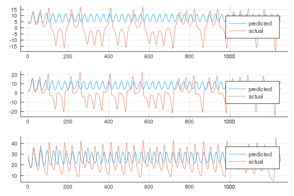
While incrementing the reservoir size is known to improve the results, up to a certain point, a smaller one will almost surely worsen them.

approx_res_size = 60

As we can see, the choice of the parameters is of the upmost importance in this model, as it is in most models in the field of Machine Learning. There are ways of searching the optimal parameters in the state space such as grid search or random search, though experience with the model will give you the ability to know what to thinker with most of the times.

If you have any questions regarding the model, the package or you have found errors in my post, please don’t hesitate to contact me!

Citing

Part of the work done for this project has been published. If this post or the ReservoirComputing.jl software has been helpful, please consider citing the accompanying paper:

@article{JMLR:v23:22-0611,
  author  = {Francesco Martinuzzi and Chris Rackauckas and Anas Abdelrehim and Miguel D. Mahecha and Karin Mora},
  title   = {ReservoirComputing.jl: An Efficient and Modular Library for Reservoir Computing Models},
  journal = {Journal of Machine Learning Research},
  year    = {2022},
  volume  = {23},
  number  = {288},
  pages   = {1--8},
  url     = {http://jmlr.org/papers/v23/22-0611.html}
}

References

[1]

Jaeger, Herbert. “The “echo state” approach to analysing and training recurrent neural networks-with an erratum note.” Bonn, Germany: German National Research Center for Information Technology GMD Technical Report 148.34 (2001): 13.

[2] Maass W, Natschläger T, Markram H. Real-time computing without stable states: a new framework for neural computation based on perturbations. Neural Comput. 2002;14(11):2531‐2560.

[3] Konkoli Z.: Reservoir Computing. In: Meyers R. (eds) Encyclopedia of Complexity and Systems Science. Springer, Berlin, Heidelberg (2017)

[4] Schiller, Ulf D., and Jochen J. Steil. “Analyzing the weight dynamics of recurrent learning algorithms.” Neurocomputing 63 (2005): 5-23.

[5] Chattopadhyay, Ashesh, et al. “Data-driven prediction of a multi-scale Lorenz 96 chaotic system using a hierarchy of deep learning methods: Reservoir computing, ANN, and RNN-LSTM.” arXiv preprint arXiv:1906.08829 (2019).

[6] Yildiz, Izzet B., Herbert Jaeger, and Stefan J. Kiebel. “Re-visiting the echo state property.” Neural networks 35 (2012): 1-9.

[7] Lukoševičius, Mantas. “A practical guide to applying echo state networks.” Neural networks: Tricks of the trade. Springer, Berlin, Heidelberg, 2012. 659-686.

[8] Lukoševičius, Mantas, and Herbert Jaeger. “Reservoir computing approaches to recurrent neural network training.” Computer Science Review 3.3 (2009): 127-149.

[9] Lu, Zhixin, et al. “Reservoir observers: Model-free inference of unmeasured variables in chaotic systems.” Chaos: An Interdisciplinary Journal of Nonlinear Science 27.4 (2017): 041102.

[10] Pathak, Jaideep, et al. “Using machine learning to replicate chaotic attractors and calculate Lyapunov exponents from data.” Chaos: An Interdisciplinary Journal of Nonlinear Science 27.12 (2017): 121102.